iFit: Optimizers: Optimization methods

Description of the optimization process and general syntax
1. Optimizers syntax
2. Optimization quality (parameter uncertainty)
Recommended optimizers
1. In short, for continuous problems: Powell (fminpowell)
2. In short, for noisy problems: Particle Swarm Optimization (fminpso)
List of optimizer implemented in iFit/Optimizers
Benchmarking Optimization methods
Model parameter constraints and additional arguments
References

Commands we use in this page: fminsearch, and many other compatible optimizers

Description of the optimization process and general syntax

The Optimizers sub-library provides a set of minimization routines, that is computational methods which attempt to minimize, in d dimensions, an objective function, often referred as the criteria or cost function, by varying a set of parameters p :

minimizer: { vary vector p ∈ ℜ^d so that objective(p) is minimal }

A usual cost function is the least-square between the model and the data. The syntax which all of these optimizers use is the one from the default Matlab fminsearch function :

>> [parameters,criteria,message,output] = fmin(objective, guess, options)

where the input arguments are:

objective: the name of the function to minimize, objective(p). This can be a string or a function handle, or an iFunc model.
guess: the starting parameter set that the objective depends on (this is e.g. a vector of numerical values).
options: a configuration structure as obtained from optimset

The optimizer, here 'fmin', can be replaced with any optimizer in the list below. The objective function should use the vector of parameters in order to compute a value (the criteria) to minimize.

objective(p)

This value is usually a positive scalar that should tend towards zero. When the objective returns a vector, the sum of its elements is used as criteria, except for the Levenberg-Marquardt for which it is used as is.

The options structure may contain the following members, in agreement with 'optimset':

options.Display: Level of display [ off | iter | notify | final ]. Default is 'off'
options.MaxFunEvals: Maximum number of function evaluations allowed, sometimes referred as the 'cost' or 'budget'.
options.MaxIter: Maximum number of iterations allowed
options.TolFun: Termination tolerance on the function value (absolute value or change). Use 'x%' to specify a relative function change, e.g. '1%'.
options.TolX: Termination tolerance on parameter change. Use 'x%' to specify a relative parameter change, e.g. '0.1%'.
options.OutputFcn: Name of an output function. When set, it is called at each iteration step. You may use 'fminplot', which is provided in Optimizers. Refer to the Fit page for more information about fminplot. A simpler/faster alternative is the 'fminstop' option.
options.PlotFcns: same as OutputFcn, but can be a set of function in a cell array.
options.FunValCheck: Check for invalid values, such as NaN or complex
options.MinFunEvals: when set, waits for a given number of iterations before testing for convergence

The options can be entered as a character string, which is evaluated to build a structure, such as:

options='Display=final; TolFun=1e-4; OutputFcn=fminplot';

The results from the minimizer are as follow:

parameters: is the parameter set which minimizes the objective function
criteria: is the criteria/objective value at the minimum solution
message: is the final optimization routine state
output: is a structure that holds some information gathered during the minimization procedure (see below)

The last output argument has at least the following fields:

output.algorithm: Algorithm used (char)
output.message: Message which details the final state of the optimizer (char)
output.funcCount: Number of function evaluations performed during the minimization (double)
output.iterations: Number of iterations performed during the minimization (double)

as well as the other useful fields:

output.parsBest: best optimized parameter
output.criteriaBest: best criteria value for the model
output.parsHistory: Parameter set history during optimization (double array)
output.criteriaHistory: Criteria history during optimization (double vector/array)
output.parsHistoryUncertainty: uncertainty on optimized parameters (half-width) obtained from the optimization history (vector)
output.parsHessianUncertainty: uncertainty on optimized parameters (half-width) obtained from the Hessian matrix, which is extremely sensitive to noise. Prefer the output.parsHistoryUncertainty value (vector)
output.parsHessianCovariance: Covariance matrix at the optimized solution (which diagonal is the parameter variance)
output.parsHessianCorrelation: Correlation matrix at the optimized solution (off-diagonal values larger that 0.7 indicate cross-correlated parameters)

In all supplied Optimizers optimizers cases, the optimizer can handle constraints (or more specifically restraints, that is constraints on parameters values), specified as a 4th input argument. These are often lower and upper bounds. Refer to the documentation of each minimizer for more information, and the documentation about fitting models onto data sets. The number of optimization parameters is not restricted.

As an example we may find the minimum of the Rosenbrock function (which is 0 at [ 1 1 ]):

>> banana = @(x)100*(x(2)-x(1)^2)^2+(1-x(1))^2;
>> fmin(banana, [0 0])
ans =
    0.9359    0.8723

and in order to get the whole optimisation information (uncertainty, ...) in 'output'

>> [parameters, fval, exitval, output] = fmin(banana, [0 0]);

Optimizers syntax

All of these optimizers follow the same syntax, just as the default Matlab fminsearch optimizer (which is based upon the simplex method).

>> [parameters, fval, exitval, output] = fminimfil(function, starting_parameters, options, {constraints})

where the options and output arguments are structures. All of these methods support constraints on parameters during the optimization process (see below).

The iData and iFunc fits method are wrappers to any of the Optimizers optimizers, with a specified fit criteria.

The objective function should be a function of a single parameter p.

function y=objective(p)
y = ...

In case the objective requires additional arguments, just pass them to the fits method (5th, 6th, ... arguments)

>> p=fminsce(objective, [ 0.5 1 0.01 0 ],options, constraints, additional_arguments);

assumes the objective function has syntax (see below for more details and an example)

objective(p, additional_arguments)

Last, the starting parameter 'guess' can also be specified as a structure which fields contain numbers, or as a string with members separated with the ';' character, such as in the following example:

>> p.par1=4; p.par2=5; 		% optimize two parameters with names par1 and par2. 
>> fminsce(objective, p)	% The result is also returned as a structure.
>> fminsce(objective, 'par1=4 ;par2=5')	% create the structure above and optimize...

In this case, the returned optimised parameters are also given as named structures:

>> banana = @(x)100*(x(2)-x(1)^2)^2+(1-x(1))^2;
>> fmin(banana, struct('A',0,'B',0))
ans = 
    A: 0.9499
    B: 0.9026

Optimization quality (parameter uncertainty)

An optimization procedure is associated to a criteria minimization. Once a local/global minimum has been found, the best found model parameters are returned. However, any optimization result is located in an uncertainty volume in which a small change of the parameters does not produce a change of the criteria larger than the tolerance used during the optimization procedure (options.TolX and options.TolFun).

In practice, if we assume the criteria and parameter distributions around the minimum to be roughly Gaussians, we may estimate the parameter change when the minimized criteria value is doubled (that is extended by its 'half-width') :

{ Δp so that χ²(p) < 2*min(χ²) }

This may be obtained from the optimization history, and the result is stored in output.parsHistoryUncertainty. where we use a Gaussian weighting for the parameter sets around the criteria value:

exp[ - (χ²(p)-min(χ²))²/8/min(χ²)² ]

Alternatively, if we consider the local criteria hyper-surface to be approximated by a quadratic, then the error bar is twice the inverse of the Hessian matrix at the optimized solution (which is the criteria curvature - very sensitive to noise):

Δp ∼ √[ 2 ||∂²χ² / ∂p_i∂p_j ||^-1 ]

This value is computed and stored in output.parsHessianUncertainty, and the corresponding error matrix (covariance) is stored in output.parsHessianCovariance (its diagonal square root is the projected parameter uncertainty). This step is only performed when the Hessian matrix requires less than about a minute to compute. Additionally, the output.parsHessianCorrelationindicates the cross-correlations between parameters (off-diagonal values larger that 0.7 indicate cross-correlated parameters).
The Hessian statistics are explicitly computed when options.Diagnostics='on', or when the time required for computation does not exceed about a minute. The parameter uncertainties are displayed when options.Display is set to 'final' or 'iter'.
The Hessian method is very sensitive to noise in the objective function. All these Hessian final computations (which may take time) can be skipped when using options.Diagnostics='off'.

It is possible to display the probability distribution of the parameters when computing the histogram of the parameter history. This is for instance often used after a Markov Chain Monte-Carlo strategy, but most heuristic (non-deterministic) optimisers allow to access this information. In the following example, after getting the 'output' 4-th returned argument, we plot all parameter distributions:

figure('Name',[ 'Parameter distributions ' output.optimizer ]);
M=numel(output.parsBest); m=floor(sqrt(M)); n=ceil(M./m);
index = find(output.criteriaHistory < min(output.criteriaHistory)*10); % select a portion close to the optimum
for p=1:M

subplot(m,n,p); hist(output.parsHistory(index,p));
title(sprintf('Parameter [%i] = %g +/- %g', p, output.parsBest(p), output.parsHistoryUncertainty(p)));

end

Recommended optimizers

The process of choosing a sensible optimizer can be automated by using the fmin optimizer. The objective function is analyzed and a set of best optimizers is determined, depending on the execution time, the number of parameters, and the type of objective - noisy or continuous:

>> fmin(objective, p)

When more than one optimizer is suitable, a random choice is performed, with a weighting by the success ratio and the number of function calls (optimization speed). Successive calls to fmin with the same problem to solve may result in different optimizers and solutions.

For this reason, it is often desirable to explicitly set the optimisation routine to use, with e.g.:

>> fminpso(objective, p)
>> fmin(objective, p,'optimizer=fminpso')

In short, for continuous problems: Powell (fminpowell)

The fastest methods are the Shor R-algoritm (fminralg, does not work for one parameter) and the Powell method is also a good choice (fminpowell). The Levenberg-Marquardt (fminlm) is very effective when the criteria is a vector. The genetic algorithm is the slowest of all methods.
The most efficient methods are the Swarm (fminpso) and the Powell method with local Coggins line search (fmipowell). The Hooke's (fminhooke) method is a good alternative, but it is slower than the Powell. We also recommend the Markov Chain Monte Carlo (fminmarkov) which is very robust, but slow.

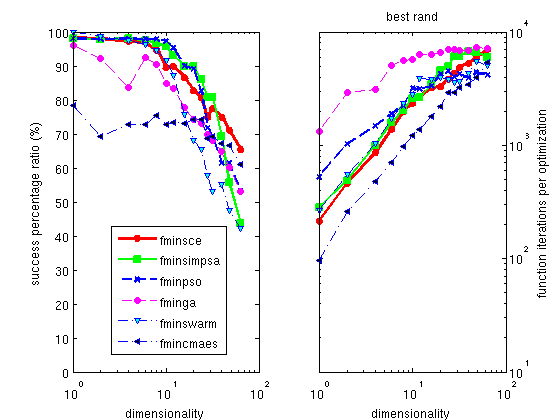
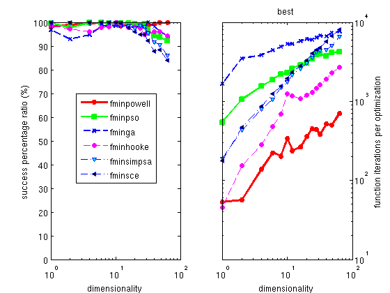
The Table 1a and Figure 1a present a selection of the 'best' optimization methods for continuous functions (non noisy problems). For each of them, we indicate the typical success ratio, and solving time (mean number of function calls required).

Figure 1a: Best optimizers for continuous (non-noisy) problems, as a function of the number of free parameters. The overall success ratio, as well as the mean execution time is shown. The Powell optimizer is both excellent in success ratio and execution time.

Optimizer	Description (continuous problems)	Mean Success ratio (%)	Cost function calls (iterations)
fminpso [8]	Particle Swarm Optimization	97.9	2757
fminpowell [13]	Powell with Coggins line search	99.21	324
fminhooke [12]	Hooke-Jeeves direct search	97.2	1177
fminimfil [3]	Unconstrained Implicit filtering	93.5	1424
fminralg [4]	Shor R-algorithm	88.9	165
fminsimpsa [1]	simplex/simulated annealing	97.1	2795

Table 1a: A selection among the most successful and fast optimization methods, for continuous (non-noisy) problems.

In short, for noisy problems: Particle Swarm Optimization (fminpso)

The fastest methods are the Evolution Strategy with Covariance Matrix Adaptation (fmincmaes) and the Particle Swarm Optimization (fminpso).
The most successful methods are the Swarm (fminpso), the Shuffled Complex Evolution (fminsce) and the simplex/simulated annealing (fmisimpsa).
For large dimensionalities (many parameters), the Evolution Strategy with Covariance Matrix Adaptation (fmincmaes) proves very successful, as well as the Shuffled Complex Evolution (fminsce). We also recommend the Markov Chain Monte Carlo (fminmarkov) which is very robust, but slow.

The Table 1b and Figure 1b present a selection of the 'best' optimization methods for noisy functions. For each of them, we indicate the typical success ratio, and solving time.

Figure 1b: Best optimizers for noisy problems, as a function of the number of free parameters. The overall success ratio, as well as the mean execution time is shown. The Particle Swarm optimizer is good in success ratio, with fair execution time.

Optimizer	Description (noisy problems)	Mean Success ratio (%)	Cost function calls (iterations)
fminpso [8]	Particle Swarm Optimization	84.1	3079
fminsimpsa [1]	simplex/simulated annealing	84.8	3672
fminsce [10]	Shuffled Complex Evolution	85.2	3184
fmincmaes [9]	Evolution Strategy with Covariance Matrix Adaptation	71.3	2066
fminimfil [3]	Unconstrained Implicit filtering	56.8	2805
fminhooke [12]	Hooke-Jeeves direct search	56.3	3067

Table 1b: A selection among the most efficient and fast optimization methods, for noisy problems.

List of optimizer implemented in iFit/Optimizers

We have performed extended tests of all the optimizers that are given in the Optimizers sub-library. For each optimizer, we have minimized a set of functions, which include sharp, broad, with local minima, etc... The function set has also been used when adding a Gaussian noise of 10%.

Each of the 52 model functions [16,17] to minimize has been solved with up to d=64 parameters.
Each of the 22 optimizers has solved all the functions, with d=1-64 parameters.
Each of these tests has been repeated 5-10 times with a random set of starting parameters.

This makes about 80000 optimizations... We then present a list of these optimizers, with their mean solving success ratio for both continuous and noisy problems. This provides a quantitative measurement of optimizers, which helps in choosing good methods, and put aside bad ones. More detailed results are shown in the table and plots below.

Generally, solving noisy problems requires longer optimization search time than for continuous problems, and the optimizers that perform best in this case are those that intrinsically make use of random numbers.

The list of all available optimizer methods can be obtained from the command:

>> fits(iData)

Function Name

Description

Success ratio
(continuous) [%]

Success ratio (noisy) [%]

Comments

fminanneal [18]

Simulated annealing

83.0

21.1

fast

fminbfgs [19]

Broyden-Fletcher-Goldfarb-Shanno

76.1

3.4

fastest gradient

fmincgtrust [5]

Steihaug Newton-Conjugate-Gradient-Trust

88.0

13.9

rather fast

fmincmaes [9]

Evolution Strategy with Covariance Matrix Adaptation

88.9

71.2

fastest swarm

fminga [15]

Genetic Algorithm (real coding)

97.2

77.6

very slow

fmingradrand [6]

Random Gradient

78.3

25.8

slowest gradient

fminhooke [12]

Hooke-Jeeves direct search

97.1

56.3

Fast and successful

fminimfil [3]

Implicit filtering

93.5

53.8

most successful gradient

fminkalman [20]

unscented Kalman filter

75.9

36.9

fminlm [7]

Levenberg-Maquardt

80.2

4.7

fminmarkov [23]
Markov Chain Monte Carlo

not bench-marked, but usually very robust

fminnewton [21]

Newton gradient search

76.7

21.3

fminpowell [13]

Powell Search with Coggins

99.2

51.7

fast and successful

Powell Search with Golden rule
options.Hybrid='Coggins'

slower than with Coggins

fminpso [8]

Particle Swarm Optimization

97.9

84.1

fminralg [4]

Shor r-algorithm

88.9

16.2

very fast

fminrand [22]

adaptive random search

74.6

62.2

fminsce [10]

Shuffled Complex Evolution

95.7

85.2

slow

fminsearchbnd [2] (fminsearch)

Nelder-Mead simplex (fminsearch)

65.8

11.5

Matlab default.

fminsimplex [14]

Nelder-Mead simplex (alternate implementation than fminsearch)

82.5

39.9

fminsimpsa [1]

simplex/simulated annealing

97.1

84.8

slow

fminswarm [11]

particle Swarm Optimizer (alternate implementation than fminpso)

95.0

75.3

slow

fminswarmhybrid [11]

Hybrid particle Swarm Optimizer

91.6

47.1

fast swarm

Table 2: Optimization methods in iFit/Optimizers, with mean success ratio in the dimensionality range d=1-64. Bold values indicate recommended algorithms. Default parameters from Matlab implementations are used, and MaxFun=2500*d, MaxIter=250*d, TolFun=1e-4. Best optimizers are highlighted in green. Methods to avoid are in red.

Benchmarking Optimization methods

Most of the optimizers given with Optimizers have been gathered from the open-source community. In a few cases, the same mathematical method has been implemented as a number of equivalent methods (swarm, simplex), but with different overall success ratios. This means that there is no unique way to code an optimization algorithm. We do not provide any guaranty regarding the effectiveness of the optimizers, but we may statistically compare them.

Swarm and Genetic algorithms

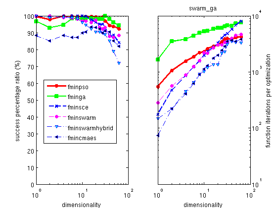
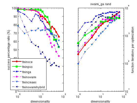
Figure 2: Mean success ratio and solving time for swarm and genetic algorithm methods, as a function of the number of parameters to optimize.

The swarm methods (aka particle swarm optimizer) provide a very good success ratio. Among these, the particle swarm optimizer fminpso is among the best. The covariance matrix adaptation evolution strategy fmincmaes has a lower success ratio but is much faster.

Gradient methods (Newton)

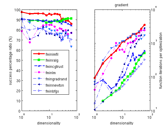
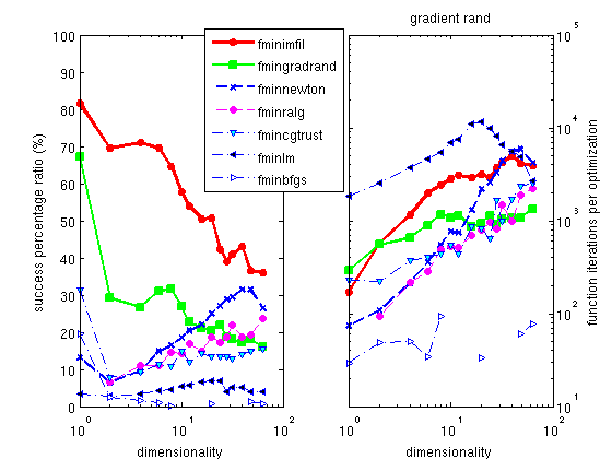
Figure 3: Mean success ratio and solving time for gradient methods, as a function of the number of parameters to optimize.

The gradient methods (derived from the Newton's method) are often considered to be the fastest. The well known Marquardt-Levenberg is an implementation of an adaptive Newton's method with a least square criteria (see below). This is true - they are fast for a reduced number of model parameters. However they often fail, as the method easily gets trapped into local minima. They are notoriously inefficient with noisy data.

Note: The Maquardt-Levenberg method fminlm is designed for objective functions/criteria as vectors. Its success ratio is then highly improved. However, its memory requirements and execution time for large dimensionalities are significantly higher than other methods.

Among these methods, we provide two excellent optimizers for continuous problems, the Implicit Filtering fminimfil and the Shor R-algorithm fminralg, which is slightly less efficient, but much faster. Only the Implicit Filtering should be used when optimizing noisy problems, all the other gradient methods fail...

Other optimizers (and simplex)

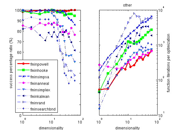
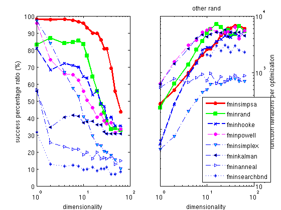
Figure 4: Mean success ratio and solving time for other non-conventional methods, as a function of the number of parameters to optimize.

The Hooke optimizer fminhooke is one of the most efficient methods for all continuous problem, and among the fastest solving time.
The Powell optimizer fminpowell is a well known, simple and efficient method, which partly works on noisy problems. Its version with the Coggins line search is the fastest of all the optimizers proposed here. The use of the Golden rule line search slightly improves its success ratio, but dramatically increases the execution time.

The default optimizer shipped with Matlab is the fminsearch one, which is a pure simplex implementation. We do not recommend this method, as all others are better in success ratio, some being as fast. A better alternative is a mix of a simplex with a simulated annealing process, implemented as fminsimpsa.

Model parameter constraints and additional arguments

In many cases, the model parameters are to be constrained. Some optimization specialists call these restraints, that is parameter values constraints. This includes some fixed values, or bounds within which parameters should be restricted. This is specified to the optimizer method by mean of a 4th input argument constraints :

>> [parameters,criteria,message,output]= fminimfil(model, initial_parameters, options, constraints)

In short, the constraints is a structure with the following members, which should all have the same length as the model parameter vector:

constraints.fixed: 1 for fixed parameter, 0 for free parameters
constraints.min: the minimum value for each parameter. -Inf is supported. NaN can be used.
constraints.max: the maximum value for each parameter. +Inf is supported. NaN can be used.
constraints.steps: the maximum change between iterations for each parameter. +Inf is supported.
constraints.eval: any other expression to evaluate, returning a modified parameter vector 'p'

All these constraints may be used simultaneously.

The constraints input argument can also be entered as a character string, like the input parameters and options :

constraints='min=[0 0 0 0]; max=[1 10 3 0.1]; eval=p(4)=0';

Fixed parameters

To fix some of the model parameters to their starting value, you just need to define constraints as a vector with 0 for free parameters, and 1 for fixed parameters, e.g. :

>> p=fminimfil(objective, starting, options, [ 1 0 0 0 ])

will fix the first model parameter. A similar behavior is obtained when setting constraints as a structure with a fixed member :

>> constraints.fixed = [ 1 0 0 0 ];

The constraints vector should have the same length as the model parameter vector.

Parameters varying within limits

If one needs to restrict the exploration range of parameters, it is possible to define the lower and upper bounds of the model parameters. This can be done by setting the 4th argument to the lower bounds lb, and the 5th to the upper ub, e.g. :

>> p=fminimfil(objective, starting, options, [ 0.5 0.8 0 0 ], [ 1 1.2 1 1 ])

A similar behavior is obtained by setting constraints as a structure with members min and max :

>> constraints.min = [ 0.5 0.8 0 0 ];
>> constraints.max = [ 1 1.2 1 1 ];

The constraints vectors should have the same length as the model parameter vector, and NaN values can be used not to apply min/max constraints on specified parameters.

Limiting parameter change

Last, it is possible to restrict the change rate of parameters by assigning the constraints.steps field to a vector. Each non-zero value then specifies the absolute change that the corresponding parameter can vary between two optimizer iterations. NaN values can be used not to apply step constraints on specified parameter.

Other constraints/restraints

The constraints.eval member can be used to specify any other constraint/restraint by mean of

either an expression making use of 'p', 'constraints',' and 'options', and returning the modified 'p' values (this expression is evaluated) ;
or a function handle of 'p', returning modified 'p' values.

For instance one could use constraints.eval='p(3)=p(1);'.

Additional arguments to the objective

If the objective function requires additional arguments (which are not part of the optimization, and are kept constant)

objective(p, additional_arguments)

the syntax for the optimization is e.g.

>> p=fminsce(objective, [ 0.5 1 0.01 0 ],options, constraints, additional_arguments);

that is additional arguments are specified as 5th, 6th... arguments. In this case, would you need to set optimizer configuration or restraints/constraints, we recommend to give 'options' and 'constraints' arguments 3-4th as structure, as explained above.

The type of the additional arguments can be anything: integer, float, logical, string, structure, cell...

For instance, we define a modified Rosenbrock 2 parameters objective which prints a star each time it is evaluated:

>> banana = @(x, cte) 100*(x(2)-x(1)^2)^2+(1-x(1))^2 + 0*fprintf(1,'%s', cte);
>> p=fminsce(banana, [ 0.5 1 0.01 0 ],'', '', '*');
.......................
ans =

    0.1592         0

References

Simplex/simulated annealing fminsimpsa [SIMPSA by Donckels] Cardoso, Salcedo, Feyo de Azevedo and Bardosa, Comp. Chem Engng, 21 (1997) 1349; Kirkpatrick, J. Stat. Phys. 34 (1984) 975.
Nelder-Mead simplex fminsearch(bnd) [fminsearch by Mathworks] Jeffrey C. Lagarias, James A. Reeds, Margaret H. Wright, Paul E. Wright, "Convergence Properties of the Nelder-Mead Simplex Method in Low Dimensions", SIAM Journal of Optimization, 9(1): p.112-147, 1998.
Unconstrained Implicit filtering fminimfil [imfil by Kelley, 1998 version] C. T. Kelley, Iterative Methods for Optimization, no. 18 in Frontiers in Applied Mathematics, SIAM, Philadelphia, 1999.
Shor's r-algorithm minimization fminralg [solvopt by Kuntsevich and Kappel] Shor N.Z., Minimization Methods for Non-Differentiable Functions, Springer Series in Computational Mathematics, Vol. 3, Springer-Verlag (1985)
Steihaug Newton-CG-Trust region algorithm fmincgtrust [cgtrust from Kelley] Broyden, C. G., J. of the Inst of Math and Its Appl 1970, 6, 76-90; Fletcher, R., Computer Journal 1970, 13, 317-322; Goldfarb, D., Mathematics of Computation 1970, 24, 23-26; Shanno, D. F.,Mathematics of Computation 1970, 24, 647-656; C. T. Kelley, 1998, Iterative Methods for Optimization no. 18 in Frontiers in Applied Mathematics, SIAM, Philadelphia, 1999.
Random gradient optimizer fmingradrand [ossrs by Belur] Computer Methods in Applied Mechanics & Engg, Vol 19, (1979) 99
Levenberg-Maquardt search fminlm [LMFsolve by Balda] Fletcher, R., (1971) Rpt. AERE-R 6799, Harwell; Fletcher, R., Computer Journal 1970, 13, 317-322
Particle swarm optimization fminpso [PSO by Donckels] Kennedy J., Eberhart R.C. (1995): Particle swarm optimization. In: Proc. IEEE Conf. on Neural Networks, IV, Piscataway, NJ, pp. 1942-1948
Evolution Strategy with Covariance Matrix Adaption fmincmaes [cmaes by Hansen] Hansen, N. and S. Kern (2004). Evaluating the CMA Evolution Strategy on Multimodal Test Functions. Eighth International Conference on Parallel Problem Solving from Nature PPSN VIII, Proceedings, pp. 282-291, Springer. ; Hansen, N. and A. Ostermeier (2001). Completely Derandomized Self-Adaptation in Evolution Strategies. Evolutionary Computation, 9(2), pp. 159-195.; Hansen, N., S.D. Mueller and P. Koumoutsakos (2003). Reducing the Time Complexity of the Derandomized Evolution Strategy with Covariance Matrix Adaptation (CMA-ES). Evolutionary Computation, 11(1).
Shuffled complex evolution fminsce [SCE by Donckels] Q. Y. Duan et al, J. of Opt. Th. and Appl. 76 (1993) 501.
Particle Swarm Optimization fminswarm and fminswarmhybrid [hPSO by Leontitsis] Kennedy J., Eberhart R.C. (1995): Particle swarm optimization. In: Proc. IEEE Conf. on Neural Networks, IV, Piscataway, NJ, pp. 1942-1948; Shi, Y. and Eberhart, R. C. A modified particle swarm optimizer. Proc. IEEE Int Conf. on Evol Comput pp. 69-73. IEEE Press, Piscataway, NJ, 1998
Hooke-Jeeves direct search fminhooke [hooke by Kelley] Arthur F. Kaupe Jr., Communications of the ACM, Vol 6. (1963) 313; R. Hooke and T. A. Jeeves, Journal of the ACM, Vol. 8, April 1961, pp. 212 ; C. T. Kelley, 1998, Iterative Methods for Optimization, no. 18 in Frontiers in Applied Mathematics, SIAM, Philadelphia, 1999.
Powell minimization fminpowell [powell by Secchi] Brent, Algorithms for minimization without derivatives, Prentice-Hall (1973)
Nelder-Mead simplex state machine fminsimplex [Simplex by Sigworth] Nelder and Mead, Computer J., 7 (1965) 308
Genetic algorithm optimizer with parameter real coding, fminga [GA by Ivakpour]
Hansen, N; Kern, S, Evaluating the CMA evolution strategy on multimodal test functions, PARALLEL PROBLEM SOLVING FROM NATURE - PPSN VIII- LECTURE NOTES IN COMPUTER SCIENCE, 3242 (2004) 282-291. [pdf]
P.N. Suganthan, N. Hansen et al, Problem definition and evaluation criteria for the CEC 2005 Special Session on Real-Parameter Optimization (2005) [pdf]
Simulated Annealing fminanneal fminanneal by joachim.vandekerckhove@psy.kuleuven.be Kirkpatrick, S., Gelatt, C.D., & Vecchi, M.P. (1983). Optimization by Simulated Annealing. Science, 220, 671-680
Broyden-Fletcher-Goldfarb-Shanno fminbfgs by A.R. Secchi Broyden, C. G., J. of the Inst of Math and Its Appl 1970, 6, 76-90 ; Fletcher, R., Computer Journal 1970, 13, 317-322 ; Goldfarb, D., Mathematics of Computation 1970, 24, 23-26 ; Shanno, D. F.,Mathematics of Computation 1970, 24, 647-656
Unscented Kalman filter fminkalman by Yi Cao Kalman, R. E. "A New Approach to Linear Filtering and Prediction Problems", Transactions of the ASME - J. of Basic Engineering Vol. 82: pp. 35 (1960)
Newton search fminnewton by C.T. Kelley Kelley 1998, Iterative Methods for Optimization, no. 18 in Frontiers in Applied Mathematics, SIAM, Philadelphia, 1999. ; W. Press, Numerical Recipes, Cambridge (1988)
Adaptive random search fminrand by A.R. Secchi 2001 A.R. Secchi and C.A. Perlingeiro, "Busca Aleatoria Adaptativa", in Proc. of XII Congresso Nacional de Matematica Aplicada e Computacional, Sao Jose do Rio Preto, SP, pp. 49-52 (1989).
Markov Chain Monte Carlo fminmarkov by Aslak Grinsted 2015. Goodman & Weare (2010), Ensemble Samplers With Affine Invariance, Comm. App. Math. Comp. Sci., Vol. 5, No. 1, 65-80

E. Farhi - iFit/optimization methods - Aug. 22, 2017 1.10 - back to Main iFit Page

Function Name	Description	Success ratio (continuous) [%]	Success ratio (noisy) [%]	Comments
fminanneal [18]	Simulated annealing	83.0	21.1	fast
fminbfgs [19]	Broyden-Fletcher-Goldfarb-Shanno	76.1	3.4	fastest gradient
fmincgtrust [5]	Steihaug Newton-Conjugate-Gradient-Trust	88.0	13.9	rather fast
fmincmaes [9]	Evolution Strategy with Covariance Matrix Adaptation	88.9	71.2	fastest swarm
fminga [15]	Genetic Algorithm (real coding)	97.2	77.6	very slow
fmingradrand [6]	Random Gradient	78.3	25.8	slowest gradient
fminhooke [12]	Hooke-Jeeves direct search	97.1	56.3	Fast and successful
fminimfil [3]	Implicit filtering	93.5	53.8	most successful gradient
fminkalman [20]	unscented Kalman filter	75.9	36.9
fminlm [7]	Levenberg-Maquardt	80.2	4.7
fminmarkov [23]	Markov Chain Monte Carlo			not bench-marked, but usually very robust
fminnewton [21]	Newton gradient search	76.7	21.3
fminpowell [13]	Powell Search with Coggins	99.2	51.7	fast and successful
	Powell Search with Golden rule options.Hybrid='Coggins'			slower than with Coggins
fminpso [8]	Particle Swarm Optimization	97.9	84.1
fminralg [4]	Shor r-algorithm	88.9	16.2	very fast
fminrand [22]	adaptive random search	74.6	62.2
fminsce [10]	Shuffled Complex Evolution	95.7	85.2	slow
fminsearchbnd [2] (fminsearch)	Nelder-Mead simplex (fminsearch)	65.8	11.5	Matlab default.
fminsimplex [14]	Nelder-Mead simplex (alternate implementation than fminsearch)	82.5	39.9
fminsimpsa [1]	simplex/simulated annealing	97.1	84.8	slow
fminswarm [11]	particle Swarm Optimizer (alternate implementation than fminpso)	95.0	75.3	slow
fminswarmhybrid [11]	Hybrid particle Swarm Optimizer	91.6	47.1	fast swarm