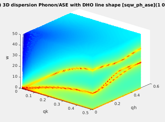
iFit: Models Phonons (fit models)
Commands we use in this page:
sqw_phonons,
iFunc
Phonon
dispersion from ab-initio force estimate and dynamical
matrix
The sqw_phonons model computes phonon dispersions
(lattice dynamics) using the Atomic Simulation
Environment (ASE) in the so-called small displacement
methodology. The only needed input for the model to run is the
name of a configuration file describing the material lattice and
atom positions. This file can be in any ASE
supported format, e.g. POSCAR,
CIF,
PDB, ... This model
requires to install external software on the computer. See Requirements (and
Installation) below.
You are also advised to
read the dedicated Phonons Tutorial.
This documentation lists all possible options.
S(q,w)
|
Description
|
Dimensionality
|
Parameters
|
sqw_phonons

|
Phonon dispersions from the Dynamical matrix,
using forces estimated by ab-initio using ASE and a
selection of DFT codes (EMT, GPAW, ABINIT, Elk,
QuantumEspresso, VASP). |
4D (HKLw)
 |
Creation: POSCAR,
CIF,
PDB, ...
Then, only the DHO line shape. ab-initio implies no
(few) tunable parameter. Axes in rlu. |
The procedure is entirely automatic. A supercell is automatically
generated, then forces are estimated by differentiation of a set of
atom displacements. Temporary data files are created. The model can
then be evaluated onto an HKLE trajectory, and plotted.
A few
words about the theory
Let us consider a perfect crystal, at very low temperature, in the
harmonic approximation close to its equilibrium. The dynamical
matrix D is defined as:
Dαβ=1/√(MαMβ)
∂2V/(∂uα∂uβ)
where V is the inter-atomic potential, M is
the atom mass, αβ are atom indices, u is
the displacement of these atoms around their equilibrium position.
The equation of motions is then:
d2uα/dt2
= - ∑ Dαβ.uβ
In order to simplify this expression, we assume a periodic motion:
uα=Uα(k)
e i(k.r - ωt)
where r is the position of the atom in a so-called super-cell,
which replicates the lattice primitive cell, and its extent sets the
potential extension distance, which is assumed to vanish at long
distance. k and ω are the momentum and energy of the
wave.
The methodology is then to displace each atom by a small quantity,
then compute the Hellmann-Feynman force F acting on
the atom to restore the equilibrium. This step is commonly achieved
by an ab-initio
code such as VASP, ABINIT and QuantumEspresso. Then
the potential partials ∂2V/(∂uα∂uβ)
are estimated by differentiating the forces as F =
-∇V after displacing atoms by small quantities. Finally, the
dynamical matrix is computed for each desired wave-vector k,
and its eigen-modes are extracted. Currently, there are a few
packages which do perform the dynamical matrix estimate and
diagonalisation steps, among which PHON, PHONON, ASE and PhonoPy. We here use
ASE together with PhonoPy (when available).
In addition, once the phonon spectrum is known, we can compute the
coherent vibrational density of states g(ω)
as, for each energy ω, the number of phonon modes lying
within a frequency [ω-dω : ω+dω] for
all wavevectors. The density of states is normalised to the total
number of modes:
∫g(
ω) d
ω = 3N
The neutron scattering intensity of the vibrational modes is
evaluated as (with a damped harmonic oscillator line shape)
I(Q,ω) ~ Amplitude *
∑ |F(Q)|2 DHO(ω0,Γ)
[n(ω)+1] / ω0
|F(Q)|2 = | ∑ bcoh
e -W(Q)|Q.e|2
e-iQ.r |2
where
e is the phonon mode polarisation vector
(multiplied by √mass), ω
0 is the mode normal
frequency,
bcoh is the coherent
neutron scattering length,
W(Q) is the Debye-Waller
function, and
n(ω) is the Bose factor
(population). The DHO line shape will be centered around the
energy Ω
2 = ω
2 + Γ
2 and Γ is
the mode damping, which holds the imaginary part of the phonon
frequency (when becoming unstable/negative).
The Debye-Waller function is estimated as:
W(Q) = ∑ |Q.e|2
[2n(ω0)+1] / 4ω0
The form factor evolves roughly as e
-1/2 <u^2>Q^2
|Q|
2 which indicates that at low and large Q,
the phonon modes are not intense. In the first Brillouin zone
(e.g. HKL < 0.5), the transverse modes are not measurable
with neutrons as |
Q.e| is null when the transverse
polarisation vector
e is perpendicular to Q. The
Amplitude
parameter includes the incoming neutron flux
I0,
detector efficiency, etc...
Amplitude ~
I0
kf/ki
where kf and ki
are the final and incident neutron wavevectors.
Syntax
The simplest syntax to create the model is to call:
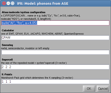 s = sqw_phonons;
% displays an entry dialog box
and proceeds with a fully automatic computation, and plots final
results. With QuantumEspresso, a dialog may show up to select
pseudo-potentials when there is more than one possibility.
The general syntax for creating the S(q,w) model is any of:
s = sqw_phonons('defaults');
% creates a simple fcc Al model and QE
as calculator
s = sqw_phonons(configuration);
s = sqw_phonons(configuration,
options, ...);
s = sqw_phonons(configuration,
calculator, options, ...);
The result is a 4D S(hkl,w) phonon dispersion Model (iFunc object).
You may as well re-import a previous calculation from its
directory, with:
s = sqw_phonons(directory);
Such a directory may contain a POSCAR* file, any previous lattice
definition (atoms.pkl as an ASE Atoms object), phonon and
vibrational calculation steps, as well as PhonoPy FORCE_SETS and
yaml files.
In addition, a web based interface can be
set up very easily by installing, on a Debian-type system, the ifit-web-services
package, and then browse to e.g. http://localhost/ifit-web-services.
Once created, we recommend to save the model with:
>> save 'my_model'
model
You can later load this model again within iFit, without the need to
recompute forces (which may be a long process with DFT codes).
>> load 'my_model'
The model parameters, once built, are the following:
p( 1)= Amplitude
p( 2)= Gamma Damped Harmonic Oscillator
width in energy [meV]
p( 3)= Background
p( 4)= Temperature [K] used to compute
the Bose factor n(w)
p( 5)= Energy_scaling
The axes needed for the evaluation are expressed in rlu for
QH,QK,QL and in meV for the energy [1 meV = 241.8 GHz = 11.604 K =
0.0965 kJ/mol]. The model can be evaluated by giving axes and model
parameters (see examples below).
- When all axes are given as vectors of same orientation and
same length, the HKLE set is assumed to be list of 'events'.
- When the H K L axes are vectors of same length/orientation,
the HKL locations is assumed to be a q-path in the BZ, but the E
(energy) axis can be of different length/orientation to compute
the Model along (q,E) path, resulting in a 2D object. Typically,
the band_structure function does this, to provide the
phonon dispersion curve along principal directions.
- When the H K L E axes are given as mixed orientations/length,
as vectors or matrices, the Model evaluation is done on a HKLE
cube, which is well suited to visualize the whole dispersion
surfaces. In the example below, ql has a
different orientation (it is transposed) as qh and qk,
which triggers a 4D HKLE cube evaluation.
- When the qh,qk,ql axes span over a whole Brillouin
zone, e.g. [-0.5 : 0.5], the phonon density of states
(DOS) is computed, and stored in s.UserData.DOS, as well
as partial DOS in s.UserData.DOS_partials (per mode).
- The maximum phonon energy is stored as s.UserData.maxFreq
- You may evaluate the powder dispersion using the powder(s)
call.
- The thermo-chemistry quantities can be obtained with the thermochemistry(s)
call.
The resulting iData object can then be plotted, such as in the following example
(grid max energy 50 meV):
	>> qh=linspace(0.01,.5,50);qk=qh; ql=qh; w=linspace(0.01,50,51);
 	>> f=iData(s,[],qh,qk,ql',w); 		% evaluate model into an iData.
 	>> plot3(log(f(1,:,:,:)));		% plot QH=0 plane
The system
configuration (atoms, unit cell)
The configuration is the location of any file format
supported by ASE, which describes the system geometry (atom types
and positions in the cell). In addition, the system configuration
can be given as a bulk, molecule, crystal and nano-tube constructors
from ASE.
configuration
|
Description
|
a file name
[ ifitpath 'Data/POSCAR_Al']
|
Any file in a format supported by ASE,
including CIF, ETSF, Gromacs, LAMMPS, PDB, SHELX,
VASP/POSCAR, MaterialStudio, XYZ. See full
list. You can use as example (provided in iFit Data
directory):
POSCAR_Al
POSCAR_AlN
POSCAR_MgO
POSCAR_Si
POSCAR_NaCl
POSCAR_SrTiO3
|
a COD ID
'cod: 1512124'
|
It is possible to retrieve a Crystallography Open
Database (COD) entry by specifying its COD ID.
This
feature requires a valid network connection. See more
details here. |
a chemical formula
'cod: O3
Sr Ti' |
It is possible to retrieve a Crystallography Open
Database (COD) entry by specifying its chemical
formula, in Hill
notation, i.e C and H first, then other elements in
alphabetical order. A search is made on COD, and when
multiple matches are found, a dialogue box pops-up to choose
a structure from a list. This feature requires a valid
network connection. See more details here. |
'bulk("Cu",
"fcc", a=3.6, cubic=True)'
|
A bulk material, with formula (Cu, MgO,
NaCl), lattice constant and structure (sc, fcc, bcc, hcp,
diamond, zincblende, rocksalt, cesiumchloride, fluorite or
wurtzite). See description of bulk.
bulk("Cu", "fcc", a=3.6)
|
'molecule("isobutane")'
|
Any molecule
known to ASE, e.g. 'isobutene',
'CH3CH2OH', 'CH3COOH', 'COF2', 'CH3NO2', 'CF3CN',
'CH3OH', 'CCH', 'CH3CH2NH2', 'PH3', 'Si2H6', 'O3', 'O2',
'BCl3', 'CH2_s1A1d', 'Be', 'H2CCl2', 'C3H9C', 'C3H9N',
'CH3CH2OCH3', 'BF3', 'CH3', 'CH4', 'S2', 'C2H6CHOH',
'SiH2_s1A1d', 'H3CNH2', 'CH3O', 'H', 'BeH', 'P',
'C3H4_C3v', 'C2F4', 'OH', 'methylenecyclopropane',
'F2O', 'SiCl4', 'HCF3', 'HCCl3', 'C3H7', 'CH3CH2O',
'AlF3', 'CH2NHCH2', 'SiH2_s3B1d', 'H2CF2', 'SiF4',
'H2CCO', 'PH2', 'OCS', 'HF', 'NO2', 'SH2', 'C3H4_C2v',
'H2O2', 'CH3CH2Cl', 'isobutane', 'CH3COF', 'HCOOH',
'CH3ONO', 'C5H8', '2-butyne', 'SH', 'NF3', 'HOCl',
'CS2', 'P2', 'C', 'CH3S', 'O', 'C4H4S', 'S', 'C3H7Cl',
'H2CCHCl', 'C2H6', 'CH3CHO', 'C2H4', 'HCN', 'C2H2',
'C2Cl4', 'bicyclobutane', 'H2', 'C6H6', 'N2H4',
'C4H4NH', 'H2CCHCN', 'H2CCHF', 'cyclobutane', 'HCl',
'CH3OCH3', 'Li2', 'Na', 'CH3SiH3', 'NaCl', 'CH3CH2SH',
'OCHCHO', 'SiH4', 'C2H5', 'SiH3', 'NH', 'ClO', 'AlCl3',
'CCl4', 'NO', 'C2H3', 'ClF', 'HCO', 'CH3CONH2',
'CH2SCH2', 'CH3COCH3', 'C3H4_D2d', 'CH', 'CO', 'CN',
'F', 'CH3COCl', 'N', 'CH3Cl', 'Si', 'C3H8', 'CS', 'N2',
'Cl2', 'NCCN', 'F2', 'CO2', 'Cl', 'CH2OCH2', 'H2O',
'CH3CO', 'SO', 'HCOOCH3', 'butadiene', 'ClF3', 'Li',
'PF3', 'B', 'CH3SH', 'CF4', 'C3H6_Cs', 'C2H6NH', 'N2O',
'LiF', 'H2COH', 'cyclobutene', 'LiH', 'SiO', 'Si2',
'C2H6SO', 'C5H5N', 'trans-butane', 'Na2', 'C4H4O',
'SO2', 'NH3', 'NH2', 'CH2_s3B1d', 'ClNO', 'C3H6_D3h',
'Al', 'CH3SCH3', 'H2CO', 'CH3CN'
molecule("H2O")
|
'nanotube(6,
0, length=4)'
|
A 1D carbon (or other material) nanotube. See
description of nanotube.
|
'crystal(...)'
|
The generic crystal builder from ASE. See
description here.
NaCl:
crystal(["Na", "Cl"], [(0, 0, 0), (0.5, 0.5, 0.5)], spacegroup=225, cellpar=[5.64,5.64,5.64, 90, 90, 90])
Rutile:
crystal(["Ti", "O"], basis=[(0, 0, 0), (0.3, 0.3, 0.0)], spacegroup=136, cellpar=[4.6,4.6,2.95, 90, 90, 90])
|
The different possibilities to specify an
atomic system/molecule in sqw_phonons.
You may look at the following resources to get material structure
files:
- MaterialsProject<https://www.materialsproject.org/>
using VASP. A. Jain*, S.P.
Ong*, et al, APL Materials, 2013, 1(1), 011002. doi:10.1063/1.4812323
- PhononDB <http://phonondb.mtl.kyoto-u.ac.jp/>
using PhonoPy and VASP. Makes use of the MaterialsProject.
- NoMaD repository <http://nomad-repository.eu/cms/>
can store any computational result from e.g. ABINIT,
QuantumEspresso, VASP, and others.
- ICSD Inorganic Crystal Structure Database <http://icsd.ill.fr> with
plenty of CIFs. requires a license.
- AflowLib <http://aflowlib.org/>
a calculation service using ICSD materials.
- COD <Crystallography
Open Database> now contains nearly 400 000 structures,
free access.
Choosing a
calculator (DFT code)
The sqw_phonons model may use any of the calculators
listed below:
'calculator=...'
|
Description
|
time elapsed [s]
|
Delta [meV/atom] |
 VASP VASP
|
Plane-wave PAW code. Used in
spin polarized mode. Requires a specific license.
|
525 (4.6)
|
|
 QuantumEspresso QuantumEspresso |
Density-functional theory, plane waves, and
pseudopotentials based code for electronic-structure
calculations and materials modeling. Used in spin
polarized mode. |
87
|
SSSP: 0.3 |
 ELK ELK |
Full Potential-All Electrons LAPW code. Used
in spin polarized mode. A very efficient
all-electrons code. Slow but reliable.
|
9820
|
0.3 |
 ABINIT ABINIT |
Plane-wave pseudopotential code. Can be used
with JTH
and GBRV
pseudo lib (nsteps=100 ecut=1000 eV)
|
64-87
|
pps=pawxml
(JTH): 0.4
pps=paw (GBRV): 0.8
pps=HGH.k: 2.1
|
 GPAW GPAW
|
Real-space/plane-wave/LCAO PAW code.
|
465
|
1.5
|
 EMT EMT |
Effective Medium Theory calculator (only
for Al,Cu,Ag,Au,Ni,Pd,Pt,H,C,N,O). Very fast, but
limited.
|
0.9
|
|
Octopus
|
Used in spin polarized mode. |
|
|
Siesta
|
Used in spin polarized mode. |
|
|
The available calculators in sqw_phonons.
We recommend VASP, QuantumEspresso, and Elk. The
computation time is given for (Al a=5.6) with 24 cores
(2.8GHz), kpoints=4, supercell=3, ecut=default, and 'accurate'
setting (using PhonoPy). These times depend on the pseudo
potential used, and are only given as estimates.
Benchmarks indicate that, for phonon dispersions:
- Quantum Espresso
is the fastest, with excellent parallelization and accuracy.
- ABINIT, VASP and GPAW are also very
efficient codes. VASP is solid rock. Results with ABINIT and
GPAW may be unstable.
- The all-electrons ELK code is about 10
times slower than QuantumEspresso, but provides reasonable
results.
- Using k-points=4 is both fast and ensures a reasonable
accuracy in phonons.
- Similarly, a supercell=3 is necessary for small
lattice cells, but 2 could be enough for large ones.
- Phonon dispersions are not too sensitive on the energy
cut-off. ecut=340 eV is satisfactory. The computational
time increases as ecut1.6 for ecut
within 200 and 1500 eV, according to our benchmarks.
- Elk can not handle large supercells without recompiling. The
Debian package we provide is done so.
- Elk is hardly sensitive to the energy cut-off in results and
computational needs.
- NWChem and Dacapo calculators are not supported as they do not
provide reliable results for phonon calculations.
- Refer to https://molmod.ugent.be/deltacodesdft
for codes comparison. Currently, best codes are QE with SSSP,
Elk, Abinit with PAWXML JTH or GBRV, GPAW. VASP 5.2 with PAW2015
GW is also excellent (when available).
Other calculators
It is also possible to use any ASE compliant calculator setting
the 'options' fields 'calculator' and 'declaration', as well as
the path to the calculator executable in the corresponding ASE
command. Use double quotes strings ("...") if needed within the
Python expressions.
- options.declaration = 'from
ase.calculators.lammpsrun import LAMMPS';
- options.calculator='LAMMPS()';
- setenv('LAMMPS_COMMAND','/usr/bin/lammps');
- s=sqw_phonons('lattice', options)
Options to specify executable locations
It is possible to indicate which executable should be used, rather
than using the default system ones.
- options.calculator
Python/ASE calculator
(see above)
- options.command='exe' Path
to calculator executable and command line, e.g. 'mpirun -np 24
vasp' to override the default
Single calculator executables can be specified for
'python','mpirun','gpaw','elk','abinit',
'quantumespresso','vasp','octopus','cp2k','siesta', for instance:
which must be used at start-up.
- sqw_phonons('Al.laz', options)
You may also simply use:
- sqw_phonons('Al.laz','python=python3; quantumespress=pw.x')
which can contain full path. To change the configuration after
initial use (e.g. move from python 2 to python3), you should first
clear the configuration with:
- clear sqw_phonons
- sqw_phonons('Al.laz','python=python2.7; quantumespress=pw.x')
Configuring
the Calculator
Other options, given as strings, or as a structure, allow to
customise how to create the supercell and other computational tuning
stuff.
An example is:
>> s=sqw_phonons(POSCAR,'ABINIT','nsteps=100; occupations=smearing; ecut=1000; pps=paw;');
More options can be obtained from 'help sqw_phonons':
- target: The 'target=LOCATION'
argument can be set to save these files to a defined directory,
which must pre-exist. Without specification, a temporary
directory will be used.
- supercell: The dimension of the supercell can
be given using e.g. the 'supercell=3'
(for a 3x3x3 supercell) argument, or 'supercell=[2
3 2]'. Let supercell=0 (default) to set
automatically the supercell from the number of atoms in
the material cell as (1000/N)^(1/6).
- calculator: the calculator to use, see below.
- potentials: pseudo potential directory to use, e.g. '/usr/share/elk-lapw/species', '/usr/share/abinit/psp', '/usr/share/espresso/pseudo'.
- diagonalization: 'david'
or 'cg'. or 'rmm-diis'.
The Davidson method is faster than the conjugate-gradient but
uses more memory. The RMM-DIIS is even faster.
- autoplot: evaluates the model on QH=0 plane, and plot
it.
- mpi: The number of CPU's to use can be set with option
e.g 'mpi=4'. This option requires
e.g. OpenMPI to be
installed, and is only validated on Linux systems (sudo
apt-get install openmpi-bin). All codes support MPI. Remember
that the memory usage increases linearly with the number of
processors involved, so in practice you should have about 2GB
per CPU requested. For 16 GB available memory, you can safely
use 8 CPUs.
- command: specify the calculator executable which may
include e.g. "mpirun -np N" when applicable (and options.mpi
should not be set).
- htmlreport: when set to 1, creates a readable report as
an HTML document 'sqw_phonons.html' in the target
directory. The syntax sqw_phonons(..., 'report', ...) also works.
- optimizer: when set, performs a geometry optimization
before computing the forces. This option can be set to 'BFGS', 'LBFGS'
(low memory BFGS), 'MDMin' or 'FIRE', as explained in the ASE
Structure optimization page. If the input configuration is
not close to its equilibrium state, it is worth setting this
option. We recommend to set it to BFGS or MDMin (which are fast)
in all cases.
- accuracy: The 'fast'
choice uses the symmetry operators to lower the number of atom
displacements. The force gradient is using central difference (2
displacements +/- on each axis). The 'very
fast' option (default) halves the number of
displacements and, when available, uses PhonoPy. The
equilibrium forces are used to improve the accuracy of the force
gradient. The 'accurate' choice
is longer to execute (e.g. 3-6 times slower), and computes all
forces ignoring symmetry. All these accuracy settings display
the ETA before completion, but are limited to 256
displacements. This limit can be reached when computing
with large cells. In this case, you may use the 'single_shot' accuracy setting
which does all computations in one shot (no ETA is displayed).
This is usually a very fast solution as well.
- use_phonopy: when set to 1, or using directly sqw_phonons(...,
'phonopy', ...), the PhonoPy library
is used, which results in a 'very fast'
calculation (using forward difference force gradient), and all
available symmetry operators. This requires PhonoPy to be
available. When not available, the default 'very fast' accuracy choice will be
used (using PHON methodology).
and more specific DFT related options:
- occupations: For metallic and insulator systems, the electron
state occupations should be set by using argument 'metal' (0.3 eV)
'semiconductor' (0.1meV) or 'insulator',
or 'occupations=smearing' or 'occupations=fixed'. You can also
directly specify the smearing width as 'occupations=<value>'
assuming a Fermi Dirac distribution. The unit is eV.
- kpoints: The size of the Monkhorst-Pack grid
can be set using e.g. 'kpoints=3'
or 'kpoints=[3 4 3]'. In order to
compute realistic phonon dispersions, the k-points value should
be at least 3. Values lower should only be used for testing. The
high accuracy value for kpoints3*supercell3
is 6750/N for a N-atom cell, but you may start with smaller
values such as 1000/N. Let kpoints=0 (default) to set
automatically the kpoints from the number of atoms in
the material cell as ∛(1000/N)/supercell.
- xc: type of Exchange-Correlation functional to use,
e.g. default 'xc=PBE'. Other
choices 'LDA','revPBE','RPBE',...
- ecut: The kinetic energy cutoff for
wavefunctions can also be specified using e.g. argument 'ecut=340'. The unit is eV. A good
estimate is to use [200*the number of different atoms]. ABINIT
with paw/pawxml potentials requires larger ecut
(1000-1500eV) and nsteps (100).
- ecutrho (optional): kinetic energy cutoff for charge
density and potential. Typical=4*ecut, suitable for PAW. Larger
value improves convergence, especially for ultra-soft PP (you
should then use 8-12*ecut). Leave it undefined to let the
calculator determine it.
- nsteps (optional): max number of iterations for SCF.
Larger value improves convergence. Leave it undefined to let the
calculator determine it.
- nbands (optional): Number of valence bands for which
wavefunctions are being computed. Should be the number of
electrons /2 and for a metal, 20% more (minimum 4 more). Leave
it undefined to let the calculator determine it.
- toldfe (optional): Convergence threshold on the energy
for selfconsistency. Typical value is 1e-6. Leave it undefined
to let the calculator determine it.
Specific
options for ABINIT
We recommend the PAWXML PBE JTH and PAW PBE GBRV potentials.
- iscf: type of self-consistent cycle. Can be 'NC' (norm-conserving) and 'PAW'.
- potentials: can be a directory path, as well as also
one of 'NC' 'fhi' 'hgh' 'hgh.sc' 'hgh.k'
'tm' 'paw' 'pawxml'
which is then sent to pps below..
- pps: Type of pseudo potential database, any of
- 'fhi' Fritz-Haber-Institute,
fast but not very accurate
- 'hgh' Hartwigsen-Goedeker-Hutter
(without semi-core valence electrons) rather fast and
moderately accurate
- 'hgh.sc' Hartwigsen-Goedeker-Hutter
(with semi-core valence electrons)
rather fast and moderately
accurate
- 'hgh.k' Hartwigsen-Goedeker-Hutter
(high k) rather fast and moderately accurate
- 'tm' Troullier-Martins
- 'paw' Projector-Augmented-Wave from ATOMPAW, very good
- 'pawxml' PAW
in XML format (from GPAW) the best, requires more iterations (e.g. ecut=1500;
nsteps=100)
Specific
options for GPAW
- mode: GPAW computation
mode as Plane-Wave, Finite Difference, or LCAO (linear
combination of atomic orbitals). Can be 'pw','fd',
or 'lcao'. Default is 'pw'. The 'lcao' mode is fast for large
systems, and requires less memory.
Specific
options for Octopus
- pps: Type of pseudo potential database, any of
- 'standard' LDA only for H, Li,
C, N, O, Na, Si, S, Ti, Se, Cd
- 'hscv_pbe' Hamann-Schlueter-Chiang-Vanderbilt
- 'hscv_lda' Hamann-Schlueter-Chiang-Vanderbilt
- 'hgh_lda' (Hartwigsen-Goedecker-Hutter
LDA pseudopotentials for elements from H to Rn)
- 'sg15' (Optimized
Norm-Conserving Vanderbilt PBE up to Bi, no Lanthanides)
Specific
options for Siesta
- potentials: should be defined as a path to a
directory containing the pseudo-potentials, e.g. '/usr/share/siesta/pseudo/'
- pps: Type of pseudo potential database, any of
- 'fhi' Fritz-Haber-Institute
(from ABINIT).
- 'tm' Troullier-Martins (from NNIN).
Specific
options for VASP
- pps: can be a structure to define explicitly which
flavour of pseudo-potentials have to be used, per element, such
as
struct('K','_pv', 'Ca', '_pv', 'Rb', '_pv', 'Sr',
'_sv', 'Y', '_sv', 'Zr', '_sv', 'Nb', '_pv', 'Cs',
'_sv', 'Ba', '_sv', 'Fr', '_sv', 'Ra', '_sv', 'Sc', '_sv')
or better struct('B','_h','C','_h','N','_h','O','_h','F','_h','H','_h','Li','_sv','Be','_sv','Na',
'_sv','Mg','_pv','K','_sv','Ca','_sv','Rb','_sv','Sr','_sv','Cs','_sv','Ba','_sv','Sc','_sv','Ti','_pv',
'V','_pv','Cr','_pv','Mn','_pv','Fe','_pv','Ni','_pv','Cu','_pv','Y','_sv','Zr','_sv','Nb','_pv','Mo','_pv',
'Tc','_pv','Ru','_pv','Rh','_pv','Pd','_pv','Hf','_pv','Ta','_pv','W','_pv','Re','_pv','Os','_pv','Al','_h',
'Si','_h','P','_h','S','_h','Cl','_h','Ga','_h','Ge','_h','In','_d','Sn','_d','Tl','_d','Pb','_d','Bi','_d','Fr','_sv','Ra','_sv')
Convergence
issues: what to try
It is generally recommended to use the following settings for
accurate phonon band computations:
- kpoints=6 (or at least 4x4x4). kpoints=3 is
suggested for a quick estimate.
- ecut=1500 [eV]. This depends on the crystal. Try 340 eV
and gradually increase value for better accuracy.
- smearing=0.27 [eV] for most materials. This helps
convergence.
- toldfe=1e-6 [eV] or lower. The default is 1e-5 for fast
estimates.
If the SCF convergence fails, you may try:
>> s=sqw_phonons(POSCAR, 'nsteps=200; toldfe=1e-6; occupations=0.27; ecut=1500; ');
For insulators, you may also use a very small smearing, e.g. 0.01
eV.
If you are tight on the memory (e.g. the system is large), you may
try:
>> s=sqw_phonons(POSCAR, 'ecut=500; diagonalization=cg');
If the convergence can not be reached, relax the tolerance criteria
on the energy 'toldfe'. However, the default value is already very
relaxed (1e-5) and you should rather play with the other parameters.
If the phonon calculation does converge, but the results show many
unstable modes, you may try to reduce the toldfe parameter to says
1e-6 or even lower (down to 1e-8).
Other tools: powder
average, density of states, etc.
The thermo-chemistry quantities (U,F,S,Cv) can be obtained with the
thermochemistry(s) call.
The vibrational density of states can be obtained with the dos(s)
call.
The standard dispersion curve plot along principal crystal
directions can be obtained with the band_structure(s) call.
See more details here.
Powder average
Once such a 4D S(hkl,w) iFunc model has
been built, it is possible to compute the 2D powder average S(|q|,w)
using:
	>> s=sqw_phonons([ ifitpath 'Data/POSCAR_Al'],'metal','EMT');
	>> pow=powder(s); plot(log(pow));
The same procedure can be applied on an evaluated iData object out of the model.
	>> qh=linspace(0.01,3,50);qk=qh; ql=qh; w=linspace(0.01,50,51);
	>> f=iData(s,[],qh,qk,ql,w);
	>> pow=powder(f); plot(log(pow));
In both cases, when the reciprocal lattice information is found in
the object (matrix B=[a* b* c*]), the conversion from 'rlu' (e.g.
2pi/a units) to 'Angs-1' is automatically done (and this
information is stored in the Model upon creation).
Examples
A usage example is:
	>> s=sqw_phonons('bulk("Cu", "fcc", a=3.6)','EMT','metal'); 	% create model from bulk
	>> qh=linspace(0.01,.5,50);qk=qh; ql=qh'; w=linspace(0.01,50,51);
 	>> f=iData(s,[],qh,qk,ql,w); 		% evaluate model into an iData
	>> plot3(log(f(:,:,1,:)));		% plot ql=0 plane
To get a system with acoustic and optical modes:
	>> s=sqw_phonons([ ifitpath 'Data/POSCAR_AlN'],'EMT'); 	% create model from given POSCAR
	>> qh=linspace(0.01,.5,50);qk=qh; ql=qh'; w=linspace(0.01,50,51);
 	>> f=iData(s,[],qh,qk,ql,w); 		% evaluate model into an iData
	>> scatter3(log(f(:,:,1,:)));		% plot ql=0 plane with acoustic and optical modes
In addition, the phonon
Density of States (aka phonon spectrum) is computed, when the
model evaluation is requested on the whole Brillouin zone (HKL vary
on [-.5 : 0.5]). The results are stored in the model UserData.DOS
and UserData.DOS_partials, so that it can be viewed with
e.g. :
	>> s=sqw_phonons([ ifitpath 'Data/POSCAR_Al'],'EMT','report); 	% create model from given POSCAR and report
	>> qh=linspace(-0.5,.5,50);qk=qh; ql=qh'; w=linspace(0.01,50,51);
 	>> f=iData(s,[],qh,qk,ql,w); 		% evaluate model into an iData, and DOS, U,S,F, Cv
 	>> figure; plot(s.UserData.DOS);
The calculation of the phonon spectrum also provides an estimate of
the entropy S, Helmholtz free energy F, internal energy U and the
specific heat at constant volume Cv as a function of the
temperature. In this example, a URL pointing to the automatically
generated report is shown at the end of the procedure (e.g. wait 5
min for completion).
The plot (surf), plot3, scatter3, and slice methods
for plotting all provide nice looking rendering of volume data. See
Plot/3D page.
References
- PHON: D.
Alfe, Computer Physics Communications 180,2622-2633
(2009) [pdf].
<http://chianti.geol.ucl.ac.uk/~dario>.
- Quantum Espresso:
P. Giannozzi, et al, J.Phys.:Condens.Matter, 21,
395502 (2009). <http://www.quantum-espresso.org/>.
Pseudo-potentials.
We also recommend the SSSP
library for which we provide the quantum-espresso-sssp
Debian package.
- VASP: G. Kresse and J.
Hafner. Phys. Rev. B, 47:558, 1993. <https://www.vasp.at/>
- PhonoPy: A.
Togo and I. Tanaka, Scr. Mater., 108, 1-5 (2015) <https://atztogo.github.io/phonopy/>
- Phonon intensity estimate: H. Schober, J Neut. Res. 17
(2014) 109. DOI
10.3233/JNR-140016
Requirements
and installation
Most DFT codes require a multi-core computer with about 4Gb/core
memory. Use option e.g. 'mpi=8' to make
use of parallelization. When not given and MPI is installed, all
processors will be used by default.
Typically, a 16-cores machine allows to run simple material (e.g.
binary/ternary materials with up to 10 atoms per cell) phonon
estimates within few hours. More complex materials will require e.g.
a few days. In terms of memory, you should have 2-3 Gb per core,
that is to say 32 Gb RAM. When installed on disk, the whole system
requires less that 10 Gb, and you need some limited storage. So, in
short 100 Gb is fair.
The ASE must be
installed. Packages exist for Ubuntu/Mint/Debian, RedHat/Fedora,
OpenSUSE, MacOSX (brew), and Windows (experimental). In addition,
the hdf5storage
python package must be installed as well. External calculators (e.g.
QE, ABINIT, VASP, ...) should be installed separately.
The required software needed to perform Phonon estimates are (see
below for the installation procedure):
See below on how to install these packages. If some of the packages
are not available, or not functional, iFit-Phonons will still be
usable with the other functional parts. It is however recommended to
install most of this list.
Virtual Machine
(our recommendation)
The fastest way to have a running system for Phonon estimates using
iFit is to download our ILL/CS
Live ready-to-run system with Phonons, McStas and iFit
(standalone) all pre-installed.
Install e.g. VirtualBox, then open the OVA file. Set its memory,
CPU, etc and import the VM. Click Start. The user account is
'lambda' and its pass word is 'illill'.
Debian systems
(Ubuntu/Debian/Mint)
For Debian systems, we provide most packages at packages.mccode.org
(currently validated on Ubuntu 14.04/Debian 8 and 16.04). To install
all in one go, type (Ubuntu/Mint/Debian, replace 'xenial' by
'trusty' for 14.04 and Debian 8 systems):
% sudo apt-add-repository 'deb http://packages.mccode.org/debian stable main'
% sudo apt-add-repository 'deb http://packages.mccode.org/debian xenial main'
% sudo apt-get update
% sudo apt-get install ifit-phonons mcrinstaller libxmu6 libxt6 libxp6 libxpm4 libxc1
which is equivalent to
% sudo apt-get install ifit elk-lapw gpaw python-matplotlib mcrinstaller libxmu6 libxt6 libxp6 libxpm4
% sudo apt-get install abinit abinit-doc abinit-psp quantum-espresso quantum-espresso-sssp phon libnetcdf-dev libxc1 openmpi-bin
% sudo apt-get install abinit-psp-jth abinit-psp-gbrv python-ase-qe-spglib python-hdf5storage python-ase python-phonopy
Note: The gpaw-setups package is
named gpaw-data
in Ubuntu distributions >= 15.10. Do not install
gpaw-setups then.
If some of the packages do not install properly, you can skip them
(except iFit and ASE). Then, you will still have access to the other
calculators.
The PhonoPy
library can be used when installed. To install it, use:
% sudo apt-get install python-dev python-numpy python-matplotlib python-yaml python-h5py python-scipy

% sudo pip install phonopy
or
% sudo apt-get install python-phonopy (when using our packages.mccode.org repository)
Python3:
iFit-Phonons can be used with Python3 as well. The required
packages to install are then:
- sudo apt install python3-ase python3-hdf5storage
Option: web service. If in addition you wish to use the web
interface (which is a very simple access solution without learning
how to use the iFit-Phonons software itself), install the package
ifit-web-services:
sudo apt-get install ifit-web-services
Then open a browser and enter the URL address http://localhost/ifit-web-services
. To benefit from the email tracking (start/stop of computations)
you will need to edit the file /usr/lib/cgi-bin/computing_sqw_phonons.pl
as administrator and change the email server/account/password to
use.
Other Linux
distributions
In principle, it is possible to install the iFit Phonons
infrastructure on RedHat class systems (e.g. Fedora), either by
installing packages manually, or converting Debian packages into RPM
ones using 'alien'.
Use your package manager (e.g. yum and dnf), if
available, to install some of e.g.
python-ase, quantum-espresso, elk-lapw, gpaw, abinit.
Then install the standalone linux executable of ifit
(standalone, zip archive) from e.g. http://ifit.mccode.org/Downloads/binary/glnx64/
into e.g. /usr/local/ifit. Also install the MCRInstaller in
/opt/MATLAB. Create a link to the ifit exeutable with e.g.:
sudo ln -s /usr/local/ifit/ifit /usr/local/bin/ifit
You may try to install the ifit-web-services package from https://github.com/McStasMcXtrace/iFit-Web.
Windows 10
There are basically 2 recommended installations. The first is via
Anaconda (see below).
The second strategy is using the Windows Subsystem for Linux (WSL):
Ubuntu / Windows 10
When running Windows 10, you can install a full
Linux/Ubuntu subsystem.
Then follow the above instructions for Debian/Ubuntu and get
packages from our
Debian main repository.
Install then with e.g.:
# sudo apt-add-repository -y http://packages.mccode.org/debian stable main
# sudo update
# sudo apt install ifit mcrinstaller libxmu6 libxt6 libxp6 libxpm4 libxc1
and optionally
# sudo apt install ifit-phonons
Then launch iFit (and other commands) from the Linux subsystem
'bash':
# ifit
Other systems:
Anaconda
Install the standalone executable of ifit (standalone, zip
archive) from e.g. http://ifit.mccode.org/Install.html
You need Python, Numpy, SciPy and MatPlotLib to be installed. For
this, we recommend that you install the Anaconda
distribution.
Install ASE, PhonoPy and QE-util using conda or pip in the Python
environment (e.g. Anaconda bash), e.g.:
conda install phonopy hdf5storage ase
conda install -c jochym qeutil
Finally, install the DFT codes referring to their documentation (see
'requirements' above). Some of the packages may not be easily
installable on MacOSX or Windows systems.
Then start the Anaconda bash and launch Matlab/iFit from there
(type: matlab or ifit at the prompt).
Python3:
iFit-Phonons can be used with Python3 as well. The required
packages to install are then:
- python3-ase python3-hdf5storage
- phonopy (optional)
Pseudo
potentials
The ABINIT code requires to install an additional library of pseudo
potentials. We recommand to get it here
(ASE) and extract it in /usr/share/abinit/. We
provide the abinit-psp
(hgh and tm) abinit-psp-jth
(pawxml) and abinit-psp-gbrv
(paw) packages for Debian. You may alternatively install for
ABINIT the package abinit-data
(which provides a limited set of pseudo-potentials).
The QuantumEspresso code requires to install an additional library
of pseudo potentials. We recommend the SSSP library for which we
provide the quantum-espresso-sssp
Debian package.
WARNING: the quantum-espresso-data
Debian package conflicts with the
quantum-espresso-sssp one. It only provides a minimal
pseudo-potential list, and is generally less accurate.
E.
Farhi
- iFit/fit models -
Nov. 27, 2018 2.0.2 -
back to
Main iFit Page 


s = sqw_phonons; % displays an entry dialog box and proceeds with a fully automatic computation, and plots final results. With QuantumEspresso, a dialog may show up to select pseudo-potentials when there is more than one possibility.
 VASP
VASP EMT
EMT