iFit: iData objects fitting
- Fitting a model to the Data
- Getting most of the fit results
(4th output argument)
- Specifying/configuring the
optimization method
- Choosing an optimization method
- Configuring the optimization
method (4th input argument)
- Monitoring the performance of
the optimization method and the fit process
- Model parameter constraints
- Fixed parameters
- Parameters varying within limits
- Limiting parameter change
- Other constraints/restraints
- Additional arguments to the
model
- Using constraints within the
model
- Estimating the model parameter
uncertainties and the fit quality
- Building model functions
- Specifying the optimization criteria
- Issues when fitting
This documentation details the procedure that can be used to find
optimal parameter set from a model in order to match (fit) an iData object Signal with axes.
fit: { vary vector
p ∈
ℜd so that
distance(Signal,
Model) is minimal }
where
distance is the
criteriion for the fit, which measures how far the model is from
the data. There is a number of possible distance definitions,
detailed
below. You can refer to
the
mathematical
optimization definition.
Fitting a model to the Data
The fits
function for iData and iFunc objects provides a simple mean to find
the best model parameters which fits a data set.
>> a=load(iData, [ ifitpath 'Data/sv1850.scn' ])
>> p=fits(a);
'Amplitude'    'Centre'    'HalfWidth'    'Background'
 0.6786         1.0008      0.0035         0.0002
will fit the data Signal/Monitor
to a default 1D Gaussian function 'gauss',
starting from automatically guessed initial model parameters. Of
course, it is possible to chose explicitly the model function, and
the starting parameter set with e.g.
>> p=fits(a, 'gauss');                    % specify model function to use: gauss, and use guessed parameters
>> p=fits(a, gauss, [ 0.5 1 0.01 0 ]);    % specify the starting parameters for the model function (3rd input arg)
The starting parameters can be given as empty (to get the current
values), as a vector, a string converted to a structure, or a
structure. When given as a structure, the resulting optimised
parameters are also returned as a structure. Unspecified parameters
are automatically guessed.
>> p=fits(a, gauss, 'Amplitude=0.5; Centre=1');
>> p=fits(a, gauss, struct('Amplitude',0.5,'Centre',1));
The two first arguments to fits are the data object (iData class) and the model object (iFunc class).
The result of the fits
method is the model parameter set that matches best the data. The
number of fit parameters is not limited.
A number of model functions is available from the Models sub-library. The list of all
available fit functions can be obtained from the
command: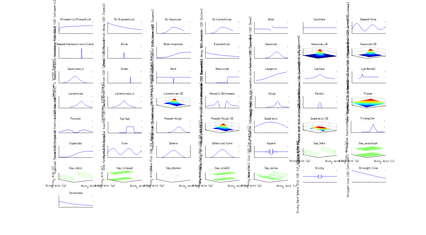
>> fits(iData); % or fits(iFunc)
Refer to the section below in order
to learn how to define new fit models with the ifitmakefunc tool, or directly
with the iFunc class. This latter supports
many operators which allow to build complex models from simpler
ones, and store them into model objects (variables). You can get
information about a model by inquiring its name. When a single input
parameter is specified, starting parameters are guessed :
>> gauss
>> disp(gauss)		% return information about the function
>> plot(gauss)		% plot the function with a default parameter set and axes
>> gauss(p, x)		% evaluate the function with parameters 'p' and axis 'x'
>> gauss(p)		% same as above with guessed axes
>> g=gauss		% g is now a variable of class iFunc
>> disp(g)
A fast way to define a new model and fit it to the data is to
directly execute, with p
the parameter vector, and x,y,...
the axes:
>> p=fits(a, 'p(1)*x+p(2)');
>> p=fits(a, @(p,x)p(1)*x+p(2)); % same with a function handle
which will transparently create the model function, and then use it
for the fit.
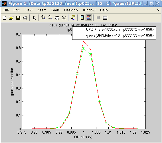 In order to estimate the values of the model
for the fit parameters onto the iData object data set axes, use the
model as argument to the object:
>> b= a(gauss, p) % evaluate the 'gauss' model onto the 'a' axes, with parameters 'p'
>> plot([ a b ])  % with parameters 'p', and plot both data and fit
In this case, the evaluated model is an iData object, which contains
Parameter and Model aliases that hold the
model parameters and description.
The fits function work
with any data and model dimensionality, and can also build
multi-dimensional models from lower dimensionality functions (e.g.
making a 2D Gaussian from multiplied orthogonal 1D Gaussians).
Warning: if you do not specify the
optimization method to use (see below),
an automatic guess is made, based on the number of parameters to fit
and the level of noise in the data and the model. As this choice is
made among a list of applicable optimizers, two consecutive fits may
chosse different optimizers and produce different fit results. In
that case, it is advisable to select a specific optimizer to use
with syntax: fits(data, model, init_pars, optimizer).
Getting most of
the fit results (4th output argument)
The fits method can return
additional arguments
>> [parameters,criterion,message,output]= fits(a, model, initial_parameters,...)
The input arguments allow to specify:
- a: an iData object,
or an array of objects
- model: the name of the function or
a function handle
- initial_parameters: a
set of starting parameters for the model. Using an empty set will trigger an automatic estimate (guess)
of the starting model parameters.
The returned arguments are similar to those returned by the Matlab fminsearch non-linear
optimizer:
- parameters: is the
best fit parameter set for the model obtained during the
optimization
- criterion: is the
criterion value (least square
χ by default - see below on how
to change this setting)
- message: is the
final optimization routine state (converged, failed, ...)
- output: is a structure that holds all
the information gathered during the fit procedure
The most interesting output argument result is the 4th one output,
which provides significantly more information such as:
- output.parsBest: best
fit
parameter set for the model
- output.criteriaBest:
best criterion value for the model
- output.modelValue: Last model
evaluation (iData), that is a(model,
parameters)
- output.algorithm: Algorithm/solver
used (char)
- output.message: Message
which
details the final state of the optimizer (char)
- output.funcCount: Number of
function evaluations performed during the fit (double)
- output.iterations: Number of
iterations performed during the fit (double)
- output.parsHistory: Parameter set
history during optimization (double array)
- output.criteriaHistory: Criteria
history during optimization (double vector/array)
- output.parsHistoryUncertainty:
uncertainty on fit parameters (half-width) obtained from
the optimization history (vector)
- output.parsHessianUncertainty:
uncertainty on fit parameters (half-width) obtained from
the Hessian matrix, which is extremely sensitive to noise.
Prefer the output.parsHistoryUncertainty
value (vector)
- output.corrcoef: fit
correlation
coefficient (closer to 1 indicates a good fit), as
obtained from Matlab corrcoef.
- output.modelName:
model name
- output.modelInfo: model
information
(structure)
- output.parsNames:
parameter names from the model
Last, the starting parameter 'guess' can also be specified as a structure which fields contain
numbers, or as a string
with members separated with the ';' character, such as in the
following example:
>> p.Amplitude=0.5; p.Center=1; p.HalfWidth=0.0035; p.Background=1e-4; 		% optimize named parameters
>> fits(a, gauss, p)								% The result is also returned as a structure.
>> fits(a,'gauss','Amplitude=0.5; Center=1; HalfWidth=0.0035; Background=1e-4')	% create the structure above and fit...
All model named parameters must be specified.
Specifying/configuring the
optimization method
The iData fits
method is a wrapper to any of the Optimizers
optimizers, with a specified fit criterion. Each optimizer can be
customized (e.g. the
maximum number of iterations, stop/convergence conditions, ...) with
an options structure.
>> [parameters,criterion,message,output]= fits(a, model, initial_parameters, options)
Choosing an
optimization method
The Optimizers sub-library provides
21 different optimization techniques. No doubt that choosing one at
first sight is difficult. We provide below a set of preferred
optimizers, based on a careful comparison explained in the Optimizers documentation.
The process of choosing a sensible optimizer can be automated by
using the fmin
optimizer (which is the default choice). The objective function is
analyzed and a set of best optimizers is determined, depending on
the execution time, the number of parameters, and the type of
objective - noisy or continuous:
>> fits(a, model, initial_parameters, 'fmin')
When more than one optimizer is suitable, a random choice is
performed, with a weighting by the success ratio and the number of
function calls (optimization speed). Successive calls to fmin with
the same problem to solve may result in different optimizers and
solutions.
Optimizer
|
Description
|
Mean Success ratio (%)
|
| fminpso |
Particle Swarm Optimization
(slow but very efficient)
|
97.9 /
84.1 |
| fminimfil |
Unconstrained Implicit
filtering
|
93.5 /
53.8
|
| fminralg |
Shor R-algorithm (avoid when
noisy) |
88.9 /
16.2
|
| fminhooke |
Hooke-Jeeves direct search |
97.1/
56.3
|
| fmincmaes |
Evolution Strategy with
Covariance Matrix Adaptation |
88.9 /
71.2
|
| fminsimpsa |
simplex/simulated annealing |
97.1 /
84.8 |
| fminsce
|
shuffled complex evolution
|
95.7 /
85.2 |
| fminpowell
|
Powell with Coggins line
search
|
99.2 /
51.7 |
fminmarkov
|
Markov Chain Monte Carlo |
robust, but slow
|
Table
1: A selection among the most efficient and fast optimization
methods. The two
success ratio are given for continuous and noisy functions resp.
The choice of the optimizer is done through a 4th input argument options
to fits (see below).
The list of all available
optimizer methods can be obtained from the command:
>> fits(iData)
Configuring the
optimization method (4th input argument)
In order to use these optimizers, one just has to specify their
names as a fits input
argument, e.g. options='fminimfil' :
>> [parameters,criterion,message,output]= fits(a, model, initial_parameters, 'fminimfil')
will select the Unconstrained
Implicit filtering coupled with BFGS fminimfil
optimizer to perform the fit. The default optimizer configuration
will be used, as obtained from the optimset function, or from the method itself with
'defaults' as
parameter. This latter call (i.e.
not with optimset) provides more information:
>> options=fminimfil('defaults') % get the default optimizer configuration parameters
The optimizer configuration
is a structure which members enable to tune the behavior of the
optimization process. Each of the fields can be changed, e.g.
>> a=load(iData, [ ifitpath 'Data/sv1850.scn' ])
>> options=fminimfil('defaults')
>> options.TolFun=0.01;
>> p=fits(a, model, [], options);	% fit with the customized options, and guessed starting parameters
The options specify the internal optimiser configuration, as
returned by optimset:
>> optimset
                Display: [ off | iter | notify | final ]
            MaxFunEvals: [ positive scalar ]
                MaxIter: [ positive scalar ]
                 TolFun: [ positive scalar ]
                   TolX: [ positive scalar ]
            FunValCheck: [ on | {off} ]
              OutputFcn: [ function | {[]} ]
               PlotFcns: [ function | {[]} ]
            Diagnostics: [ on | {off} ]
In addition to the default optimset
structure fields, the iData fits
and the Optimizers
optimizers use additional members in the structure:
- options.Display: Level
of
display [ off | iter | notify | final ]. Default is 'off'
- options.MaxFunEvals: Maximum
number of function evaluations allowed
- options.MaxIter: Maximum number of
iterations allowed
- options.TolFun: Termination
tolerance on the function value (absolute value or change). Can
be specified in '%x'
for a relative value.
- options.TolX: Termination
tolerance on parameter change. Can be specified in '%x' for a relative
value.
- options.OutputFcn: Name of an
output function (see below). You
may use 'fminplot', which
is provided in Optimizers. This
function should have the syntax fminplot(pars, optimValues, state).
- options.PlotFcns: same as OutputFcn, but can be
a set of function in a cell array.
- options.FunValCheck: Check for
invalid function/model values, such as NaN or complex and abort.
- options.algorithm: is a
description of the optimization method (solver)
- options.optimizer: is the name of
the optimization function (solver)
- options.criteria: the
criterion to use with syntax criterion(Signal,
Error,
Model). The default is least-square error (see below).
- options.Diagnostics:
when set to 'on'
or 1, returns the correlation coefficient and Hessian matrix
- options.MinFunEvals: when set, waits for a given number
of iterations before testing for convergence
- and more, depending on the optimizer method and implementation
The options can also be entered as a single string such as in :
>> p=fits(a, model, [], 'optimizer=fminimfil; Display=iter; OutputFcn=fminplot; TolFun=0.01;');
which avoids creating a structure.
Monitoring function, to be used in OutputFcn and PlotFcns,
are:
- fminplot to plot the criteria, and parameter space (our
best choice)
- fminstop to just display a stop button (very fast,
allow clean abort of fit)
- optimplotx plots the current point
- optimplotfval plots the function value
- optimplotfunccount plots the function count
Monitoring the
performance of the optimization method and the fit process
In order to follow the optimization process, you may define a call
to a user function at each optimization iteration. A default
plotting facility has been implemented as the fminplot
function:
>> a=load(iData, [ ifitpath 'Data/sv1850.scn' ])
>> options=fminimfil('defaults')
>> options.OutputFcn='fminplot';
>> p=fits(a, gauss, [], options)
p =

    0.6263    1.0008   -0.0037    0.0002
>> b = a(gauss, p)
>> figure; plot([ a b ])
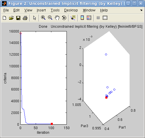
 Left:
Left: The
options.OutputFcn='fminplot' window
on
the
right,
showing
the
criterion
evolution
with
the
optimization
iteration
and
up
to
the 3 first fit parameters. The
red dot indicates the current/final parameter set
and criterion.
Right: The final fit result on the left.
Also, as explained
above, it is
possible to obtain, on optimization completion, the whole
criteria, and parameter set history, as a function of
iterations/criteria evaluations.
>> [p,criterion,message,output]= fits(a, gauss, [], options)
>> output.parsHistory
>> output.criteriaHistory
The monitoring window above can be re-displayed with:
>> fminplot(output);
Model parameter constraints
In many cases, the model parameters are to be constrained. Some
optimization specialists call these restraints, that is parameter values constraints.
This includes some fixed values, or bounds within which parameters
should be restricted. This is given to the fits method by mean of a 5th input argument constraints
:
>> [parameters,criterion,message,output]= fits(a, model, initial_parameters, options, constraints)
In short, the constraints is a structure with the following members,
which should all have the same length as the model parameter vector:
- constraints.fixed: 1
for fixed parameter, 0 for free parameters
- constraints.min: the
minimum value for each parameter. -Inf is supported. NaN can be used.
- constraints.max: the
maximum value for each parameter. +Inf is supported. NaN can be used.
- constraints.steps: the
maximum
change between iterations for each parameter. +Inf is supported.
- constraints.eval: any other expression to evaluate,
returning a modified parameter vector 'p'
All these constraints may be used simultaneously.
The constraints input
argument can also be entered as a character string, like the input parameters and options :
constraints='min=[0
0 0 0]; max=[1 10 3 0.1]; eval=p(4)=0';
As constraints apply on the iFunc model, it is possible to
manipulate all constraints using the object syntax and methods, as
explained below.
Fixed parameters
To fix some of the model parameters to their starting value, you
just need to define constraints
as a vector with 0 for free parameters, and 1 for fixed
parameters, e.g. :
>> a=load(iData, [ ifitpath 'Data/sv1850.scn' ])
>> p=fits(a, gauss, [], 'fminimfil', [ 1 0 0 0 ])
** Minimization performed on parameters:
    'Amplitude'    'Centre'    'HalfWidth'    'Background'

    0.5936    0.9998    0.0018    0.0050

p =

    0.5936    1.0008   -0.0037    0.0002
will fix the first model parameter, which is here the Amplitude. This parameter
name can be checked by simply entering the name of the model, which
returns some information structure :
>> disp(gauss)
ans = iFunc 1D model:
         Expression: @(p,x)p(1)*exp(-0.5*((x-p(2))/p(3)).^2)+p(4)
        Description: Single 1D Gaussian model
                Tag: 'iF420775'
               Date: '17-Jul-2012 15:50:11'
               Name: 'Gaussian (1D) [gauss]'
         Parameters: {'Amplitude'  'Centre'  'HalfWidth'  'Background'}
              Guess: [function_handle]
          Dimension: 1
    ParameterValues: []
           UserData: ''

Parameters:
  p(  1)=           Amplitude
  p(  2)=              Centre
  p(  3)=           HalfWidth
  p(  4)=          Background
A similar behavior is obtained when setting constraints as a
structure with a fixed
member :
>> constraints.fixed = [ 1 0 0 0 ];
>> p=fits(a, gauss, [], 'fminimfil', constraints);
The constraints.fixed vector should have the
same length as the model parameter vector.
Once the iFunc model object has been instantiated, it is possible to
fix/free its parameters with the lock/munlock methods, or
more explicitly:
>> f=gauss;			% create a Gaussian model
>> f.Amplitude = 'fix';		% fix its Amplitude. 'free' would free it
>> mlock(f, 'Amplitude')	% same as above. munlock would free it.
Parameters varying
within limits
If one needs to restrict the exploration range of parameters, it is
possible to define the lower and upper bounds of the model
parameters. This can be done by setting the 5th fits argument to the lower
bounds lb, and the 6th to
the upper ub, e.g. :
>> a=load(iData, [ ifitpath 'Data/sv1850.scn' ])
>> p=fits(a, 'gauss', [], 'fminimfil', [ 0.5 0.8 0 0 ], [ 1 1.2 1 1 ])
						lb		ub
A similar behavior is obtained by setting constraints as a structure
with members min and max :
>> constraints.min = [ 0.5 0.8 0 0 ];
>> constraints.max = [ 1 1.2 1 1 ];
>> p=fits(a, 'gauss', [], 'fminimfil', constraints);
The constraints min and max vectors should have the
same length as the model parameter vector.
Once the iFunc model object has been instantiated, it is possible to
bound its parameters with the xlim method, or more
explicitly:
>> f=gauss;			% create a Gaussian model
>> f.Amplitude = [ 0 10 ];	% bound Amplitude between 0 and 10
>> xlim(f, 'Amplitude', [0 10])	% same as above
Limiting parameter
change
Last, it is possible to restrict the change rate of parameters by
assigning the constraints.steps
field to a vector. Each non-zero value then specifies the absolute
change that the corresponding parameter can vary between two
optimizer iterations.
In short, the constraints structure can have the following members,
which all should have the same length as the model parameter vector:
- constraints.fixed: 1
for fixed parameter, 0 for free parameters
- constraints.min: the
minimum value for each parameter. -Inf is supported.
- constraints.max: the
maximum value for each parameter. +Inf is supported.
- constraints.steps: the
maximum
change between iterations for each parameter. +Inf is supported.
Other
constraints/restraints
The constraints.eval
member can be used to specify any other constraint/restraint by
mean of
- either an expression making use of 'p', 'constraints',' and
'options', and returning the modified 'p' values (this
expression is evaluated) ;
- or a function handle of 'p', returning modified 'p' values.
For instance one could use constraints.eval='p(3)=p(1);'.
All these constraints may be used simultaneously.
The constraints input
argument can also be entered as a character string, like the input parameters and options :
constraints='min=[0 0 0 0]; max=[1 10 3 0.1];
eval=p(4)=0';
NaN values in these
constraints are ignored (the corresponding parameters are not
constrained).
Once the iFunc model object has been instantiated, it is possible to
restraint its parameters explicitly with expressions:
>> f=gauss;			% create a Gaussian model
>> f.Amplitude = 'abs(p(1))';	% set Amplitude as its absolute value (Amplitude is p(1), as listed from disp(f))
>> f.Amplitude = 'abs("Amplitude")';	% same as above, double-quoting requests parameter name search in model
>> f.Amplitude = '"Amplitude" - "Background"';	% it is possible to use any parameter in expressions
Additional
arguments to the model
When defining a model with n parameters and rank m
(that is m axes), any fit process will optimize the n
parameters by evaluating the model on the m axes. If you
need to use additional arguments to the model, which are fixed
during a fit/optimization, you can access them from the 'varargin'
variable in the Expression and Constraints. varargin{1} is the
first additional argument, varargin{2} the second...
>> f=gauss;
>> disp(f)
f = iFunc 1D model:
         Expression: signal = feval(@(p,x)p(1)*exp(-0.5*((x-p(2))/p(3)).^2)+p(4), p, x);
        Description: Single 1D Gaussian model
                Tag: 'iF457990'
               Date: '16-Sep-2013 10:03:45'
               Name: 'Gaussian (1D) [gauss]'
         Parameters: {'Amplitude'  'Centre'  'HalfWidth'  'Background'}
              Guess: @(x,s)[NaN,m1(x,s-min(s(:))),m2(x,s-min(s(:))),NaN]
         Constraint: [1x1 struct]
          Dimension: 1
    ParameterValues: []
           UserData: ''

Parameters (4):
  p(  1)=           Amplitude
  p(  2)=              Centre
  p(  3)=           HalfWidth
  p(  4)=          Background

>> f([1 2 3 4], 1:10)	% evaluate with parameters p=[1 2 3 4] and axis x=1:10
ans =
    4.9460    5.0000    4.9460    4.8007    4.6065    4.4111    4.2494    4.1353    4.0657    4.0286
>> f.Constraint.eval='disp(varargin)';	% add a constraint to be evaluated, using additional arguments
>> f([1 2 3 4], 1:10, 'eee')	% evaluate again, with additional arguments
 'eee'			<-- here is displayed 'varargin' when evaluating Constraint.eval
ans =
    4.9460    5.0000    4.9460    4.8007    4.6065    4.4111    4.2494    4.1353    4.0657    4.0286
>> f.Expression=@(p,x, varargin)p(1)*exp(-0.5*((x-p(2))/p(3)).^2)+p(4)+varargin{:}
>> f([1 2 3 4], 1:10, 1)
 [1]			<-- here is displayed 'varargin' when evaluating Constraint.eval
ans =			<-- and we add it the the result as specified in the new Expression
     5.9460    6.0000    5.9460    5.8007    5.6065    5.4111    5.2494    5.1353    5.0657    5.0286
Using constraints
within the model
It may be easier to store constraints directly within the model used
during the fit. The main advantage is that constraints can be
directly related to the name of the model parameters.
To set a constraint on a model parameter, define the 'constraint'
input argument when calling fits or set the constraint directly on
the model parameters with:
>> model.parameter='fix'     % to lock its value during a fit process
>> model.parameter='clear'   % or 'free' to unlock value during a fit process
>> model.parameter=[min max] % to bound value
>> model.parameter=[nan nan] % to remove bound constraint
>> model.parameter=''        % to remove all constraints on 'parameter'
>> model.parameter='expression'        % to set the parameter from an expression
>> model.Constraint=''       % to remove all constraints
>> model.Constraint = 0;     % to unlock/free all Parameters during a fit process
>> model.Constraint = 1;     % to lock/fix all Parameters during a fit process
Any parameter name surrounded by double quotes, e.g. "Amplitude", is replaced by the
corresponding p(n) value
in an expression used for setting a parameter value
(cross-constraints). For instance
>> f=gauss;			% create a Gaussian model
>> f.Amplitude = 'fix';		% fix its Amplitude
>> f.Background = [0 1e-4];	% bound its background
>> f.Width = 'p(1)/1000';	% use an expression referring to p(1)/1000 value
>> f.Width = '"Amplitude"/1000';	% same as above with direct naming as p(1)=Amplitude
Alternatively, you can use the mlock,
munlock and xlim
methods:
>> mlock(f, {'Amplitude','Background'})	% fix these 2 parameters, same as setting parameters to 'fix'
>> munlock(f, 'Background')		% unlock that parameter, same as f.Background='clear'
>> xlim(f,    'Background', [0 1e-3])	% force parameter within range, same as f.Background=[min max]
>> xlim(f,    'Background', [])		% remove limits constraint
Last, you can fix/clear/bound parameters based on a regular
expression search such as:
>> mlock(f, regexp(f.Parameters, 'Amplitude|Background'})
where we have used the '|' OR operator.
To list parameters which are fixed, free and bounded, use:
>> mlock(f)
>> munlock(f)
>> xlim(f)
which return the number of parameters in each category.
Estimating the model parameter
uncertainties and the fit quality
Some theoretical notes about the goodness of fit are indicated
in the Optimizers help.
To get the fit statistics, you need to use the syntax:
>> [parameters,criterion,message,output]= fits(data, model, ...)
i.e. retrieve all output arguments. Then the 'output'
4-th returned argument holds lots of information.
The uncertainty on the fit parameters can be obtained from:
- output.parsHistoryUncertainty
- output.parsHessianUncertaint
Additionally, the output.parsHessianCorrelation
indicates the cross-correlations between parameters (off-diagonal
values larger that 0.7 indicate cross-correlated parameters).
The Hessian statistics are explicitly computed when options.Diagnostics='on', or when the time
required for computation does not exceed about a minute.
The parameter uncertainties are displayed when options.Display is set to 'final' or 'iter'.
The Hessian method is very sensitive to noise in the objective
function. All these Hessian final computations (which may take time)
can be skipped when using options.Diagnostics='off'.
We also explain in the Optimizers
help how the parameter distributions (their variation around
the best optimum value) can be plotted. This is well known from
heuristic optimizers and e.g. the Markov Chain Monte-Carlo.
The fit quality can be assessed from the output.corrcoef returned value which goes from 0
(very bad fit) to 1 (perfect fit). A value higher than 0.95 is
usually very good.
Building model functions
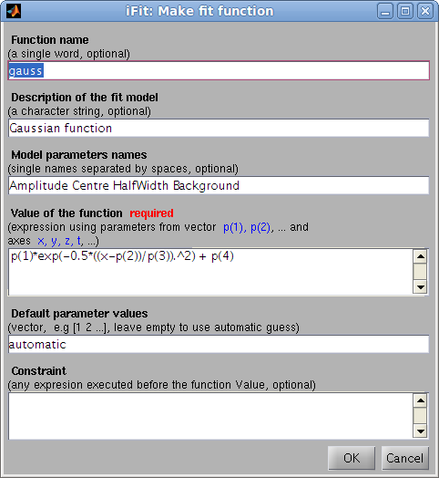 The
ifitmakefunc
tool has been designed to automatically create model functions from
either a single expression, or a more detailed description. Refer to
the Models/Model Builder.
>> h=ifitmakefunc;                              % pops-up a dialog to define the new fit function/model
>> h=iFunc('p(1)*exp( (x-p(2))/p(3) )');	% directly create an iFunc model
>> fits(a, h)
The resulting model has the ability to identify itself ('identify', provide
detailed information), compute automatic starting parameters ('guess'), display itself
('plot'), and
evaluate its value of course. It can be directly used with fits, either with their name,
or their function handle.
It is even possible to directly call the fitting method and create
the model function on the fly, which makes the fit much easier for
simple functions that can be written as a single expression:
>> fits(a, 'p(1)*exp( (x-p(2))/p(3) )'); % does the same as above, in a single command
To assemble existing functions into new ones, you may use e.g. :
>> h=gauss+lorz; h.Constraint = 'p(8)=0;';
which creates a new function which is the sum of a Gaussian and a
Lorentzian. The second redundant Lorentzian Background p(8) parameter is forced to 0
so that it does not correlate with the Gaussian Background p(4). Other function
information/parameter names (here not specified) are
guessed/defaulted.
It is even possible to convolute
and correlate functions and data sets as new function definitions.
Refer to the Models page.
In case the model requires additional arguments, just pass them to
the fits method (arguments above the 5th)
>> p=fits(a, model, [ 0.5 1 0.01 0 ],'','',additional_arguments);
assumes the model function has syntax
model(p, axes from object, additional_arguments)
Specifying the optimization criteria
The default optimization criterion is the 'least square
error':
χ2 = ∑ (Signal-Model)2.
When the Monitor is defined (see iData definition), the Signal
is normalized, so that
χ2 = ∑
(Signal/Monitor-Model)2.
When the Error on the Signal is available, the weighted criterion
reads
χ2 = ∑
[(Signal/Monitor-Model)/Error]2.
The options.criteria can be defined as the name of a criterion
function with syntax criterion(Signal,
Error, Model) where all arguments should have the same
dimension, and the default criterion is:
options.criteria =
'least_square';
% criterion definition
The Signal will be normalized to the Monitor prior to calling
the criteria. The Error is used as weight.
The criterion is then normalized to the number of degrees of
freedom by dividing it by
χ2 ← χ2
/(number_of_data_points_in_the_Signal
- number_of_parameters
-1)
The following pre-defined functions can be used as criteria:
criterion
(Signal,Error,Model) |
Expression
|
comment
|
least_square
|
(|Signal-Model|/Error)2
|
non-robust. Ref.
|
least_absolute
|
|Signal-Model|/Error
|
robust. Ref.
|
least_median
|
median(|Signal-Model|/Error)
|
robust, scalar. Ref.
|
least_mean
|
mean(|Signal-Model|/Error) |
Ref.
|
least_max
|
max(|Signal-Model|/Error)
|
non-robust, scalar. Ref.
|
least_rfactor
|
(|Signal-Model|/Error)2/(Signal/Error)2
|
non-robust. Ref.
|
max_likelihood
|
(|Signal-Model|/σ)2 + 1/2
log(2πσ) |
Ref.
Minimize -log(L).
The σ 'error' is refined during the fit. |
max_corrcoef
|
1-corrcoef(Signal, Model)
|
Ref.
|
Issues when
fitting
If you can not obtain a good fit, you can think about the
following things to do:
- redefine the data set Error,
which is used as weighting factor in the evaluation of the
criterion. The sqrt(Signal)
(default) may not be suited. Try setting a.Error=1 ;
- change the criterion definition (see above). The least square (default) may not be
suited to the Signal ; you may try the Maximum
likelihood.
- try with a specific optimizer.
The default fmin
optimizer, that makes a guess of a suitable routine may do a
wrong guess ;
- if the chosen optimizer is heuristic (that is non
deterministic), such as swarm and annealing methods, repeat
the fit. The solution will be different ;
- set constraints to model
parameters, so that they remain reasonable. In practice, set
the minimum and maximum range values. Use Nan or Inf not to
constraint a parameter ;
- set the starting parameter set to a sensible guess, rather
than relying on the automatic guess.
Good luck !
E.
Farhi
- iFit/iData fitting -
Nov. 27, 2018 $Revision: 1229 $ - back to
Main iFit Page


 The
The
