iFit: iFunc object description
The iFunc class is a
structure which holds a multi-parameter model, to be used
for e.g. plot or fit onto a data set. Models can be assembled using
standard Matlab operators. There exist a set of pre-defined Models, which you can assemble to define
more complex ones. You can also Fit an iFunc
model onto an iData object (containing
e.g. some experimental data).
The iFunc Models also exist in a set of specialized flavours
(sub-classes) which inherit full iFunc capabilities, and add
a few more specialized functionalities:
Creating and inquiring iFunc models
(iFunc, get, plot, subplot)
A model object holds an
Expression (to compute the model value), a list of parameter names,
a Guess expression to compute parameter value estimates, as well as
other MetaData just as for iData objects.
To create a model (i.e. instantiate a class into an object), specify
its Expression, using
- x,y,z,t,u,v,w: axes of
ranks 1,2, 3, 4... The 1st axis rank corresponds with rows, 2nd
for columns, ...
- p: parameter values
e.g. p(1), p(2), ...
- signal: the model
value when the Expression contains more than one statement.
For instance a linear model is obtained with
>> a=iFunc('p(1)*x+p(2)')

a =  iFunc 1D model:

    [Tag] [Dim]                                [Model] [Parameters 'p']
 iF193482   1        p(1)*x+p(2)  signal = p(1)*x+p(.. Amplitude Constant

>> a=iFunc('a=p(1); b=p(2); signal=a*x+b');	% same as above
Any expression can be entered, and an analysis of the parameters
results in default parameter names.
You can then display the full content of the object with the disp or get methods :
>> disp(a)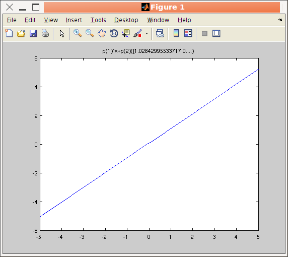
a = iFunc 1D model:
Expression: signal = p(1)*x+p(2);
Tag: 'iF193482'
Date: '17-Jul-2012 10:49:50'
Name: ' p(1)*x+p(2)'
Parameters: {'Amplitude' 'Constant'}
Dimension: 1
ParameterValues: []
UserData: ''
Parameters:
p( 1)= Amplitude
p( 2)= Constant
>> plot(a)
A graphical representation of the model is obtained using the plot method.
Properties of the model can be obtained with the get method, or with
direct indexing :
>> get(a, 'Expression')
>> a.Expression
ans =

signal = p(1)*x+p(2);
The Expression can be a
character string returning the
'signal' as a function of the parameters 'p' and axes x,y,z,t,u,v,w
It can also be given as a function handle signal=@Expression(p, x,y, ...), which usually
makes the model evaluation much faster.
>> a=iFunc(@(p,x)p(1)*x+p(2))
Additional arguments (above the model dimensionality) are usable in
the Expression as 'varargin' cell.
The name of the parameters can be changed by accessing the Parameters property (this is a
cell of strings) :
>> a.Parameters = {'Slope','Constant'}
The ParameterValues
property holds the last parameter values (e.g. when returned from a
fit or a function evaluation).
The Guess property should
return a vector of parameter values
'p' as a function of the axes x,y,z... and a signal.
This is a character string, vector or a function handle p=@Guess(x,y,z, ..., signal).
Values of the parameters left as NaN
indicate that the automatic guess procedure should be used (which is
based upon a signal peak search, and baseline analysis). The Guess
is used when starting a fit procedure for starting parameters.
Last, the Constraint
property holds any script to change the parameter values (character
string modifying 'p') from
axes x,y,z,... or a
function handle p=@Constraint(p,
x,y,...). See below on how
to define Constraints.
The model dimension, i.e. the number of axes required for its
evaluation, is stored in the Dimension property. 0=scalar,
1,2,3,4 ...
A negative dimension is used to indicate a variable dimensionality,
i.e. the model can accept more axes, or dimensionality is defined
after instantiation.
To print out the equivalent function f(p, x, ...)
from an object, convert it to a char or cellstr:
>> a=iFunc('p(1)*x+p(2)')
>> char(a)
>> cellstr(a)
Last, it is possible to define an empty iFunc object, and fill it
with Parameters and any Expression, even without actually any
mathematical model:
>> a=iFunc;
>> a.Parameters={'Amplitude','Width'}
>> a.Expression=[ '[ varargin{:} ]' ];
This way, it is possible to define any Matlab function inside an
iFunc object. The cell 'varargin' then contains the arguments 2-end,
while 'p' contains the first argument.
>> a(1,2,3)
ans =
     2     3
Accessing or
modifying parameter values
Parameters from a model can be accessed in many equivalent ways.
If 'a' is an iFunc model
:
>> a.Parameters		% lists all parameter names
>> get(a)		% display the model description, with the list of parameter names and last evaluated values
>> a.p			% returns a vector of parameter values
>> a.ParameterValues	% same as above, last evaluated parameter values
If, for instance, the model has an 'Slope' parameter, you can get specifically
its value with :
>> a.Slope % display the value of the 'Slope' parameter
Alternatively, it is possible to modify parameter values :
>> a.p(1) = 2;
>> a.Slope = 2;
Defining a new model
To define a new model with a
dialogue window, use:
>> edit(iFunc)
 Refer to the dedicated help on this topic in
the Models page, which also lists
pre-defined models (Gaussian, Lorentzian, exponential, lines,
quadratic, ...). Edit their code to see how to define new models:
>> edit gauss % edit the function definition (from a file)
>> edit voigt
>> edit(voig) % edit the object definition
When no parameter value is known, some guessed values are estimated
from the analysis of the model value and expression.
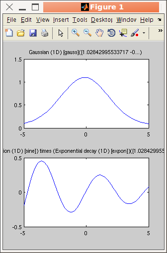
The plot method
demonstrated above can display a set of models in a single axis
frame, or a set of panels (subplot)
:
>> plot([gauss lorz])
>> subplot([gauss sine.*expon])	% use unary and binary operators, see below
Model from a
tabulated data set
It is also possible to create a model out of an iData (data
set) object. Then, the model parameters are the total intensity
scaling, as well as an offset and a scaling factor per axis. In
order to create a model from a data file, use:
>> iFunc(iData('filename'))
will create a data set object and derive a model out of it.
Evaluating a model with parameter
values and axes
The syntax for evaluating a model is
model(parameters)
% use
guessed axes
model(parameters, x,y, ...)
%
use given axes
feval(model,
parameters, x,y,z, ...)
iData(model, parameters, x,y,z,
...) % evaluate and convert into an iData
object
where parameters can be a numerical vector, or a structure with
named parameters matching the model ones, x,y,z,t,u,v,w are
axes values for ranks 1,2,3... Additional arguments (above the model
dimensionality) are usable in the Expression as 'varargin' cell.
When the parameters are specified as empty ( [] ), current parameter
values are used, or guessed. These parameters can also be given as a
vector corresponding to the model parameter order, a string such as
'Intensity=1; Width=.5', a structure
with named fields and values such as:
- p.Intensity=1;
- p.Width=0.5;
- model(p)
The evaluation of a model with a set of parameters is obtained by
calling the feval
function with the parameter values, or sending these values directly
to the object :
>> signal = feval(gauss, [ 1 0 .1 0])
>> gauss([ 1 0 .1 0])			% same as above: evaluate model
In this case, tentative axes are computed from the model definition.
Axes can also be passed as additional arguments for x,y,z,... either as separate
arguments, as a cell array {x,y,...}, as a structure, or as an iData object which axes are used.
>> feval(gauss, [ 1 0 .1 0], linspace(-5,5, 100) )
>> gauss([ 1 0 .1 0], linspace(-5,5, 100) )		% same as above: evaluate model
When used together with iData objects, the
iFunc models can either return their evaluation (array), or be
converted into an iData object for easier further handling.
>> iD = iData(linspace(-5,5, 100), zeros(1,100));	% define a zero iData object with some axes
>> g  = gauss; 						% a Gaussian model
>> g([ 1 0 .1 0], iD)					% evaluate model with axes in the iData object
>> iD(g, [1 0 .1 0])					% evaluate model into a new iData object
A faster calling syntax for the same result is:
>> g=gauss;
>> iData(g, [1 0 .1 0], linspace(-5,5, 100), zeros(1,100))	% evaluate model into a new iData object
It is also possible to evaluate the model while scanning
parameters. To achieve that, the parameter values must be
given as a named structure, or as a string such as 'Intensity=[ .5 1 1.5 2 ];'
For instance, to scan the Intensity parameter in a Gaussian,
and get the model value as an array of data sets, use:
-
model = gauss1;
-
p.Intensity= [ .5:.25:2 ]; % from 0.5 to 2 by steps of .25
-
v=iData(model, p); % evaluate as iData sets. To only get the values, use feval(model,p)
-
plot(cat(2,v)); % plot the scan as a surface
Scans with multiple parameters vectors can be performed the same
way.
Setting
and removing constraints on models
Models are often used for fitting purposes (refer to the Fit help page).
To set a constraint on a model parameter, define the 'constraint'
input argument when calling fits (see Fit)
or set the constraint directly on the model parameters with:
>> model.parameter='fix'     % to lock its value during a fit process. Same as mlock
>> model.parameter='clear'   % or 'free' to unlock value during a fit process. Same as munlock
>> model.parameter=[min max] % to bound value
>> model.parameter=[min value max] % to bound the parameter and set its value
>> model.parameter=[nan nan] % to remove bound constraint
>> model.parameter=''        % to remove all constraints on 'parameter'
>> model.parameter='expression'        % to set the parameter from an expression which can use 'p(n)' for other parameters
>> model.Constraint=''       % to remove all constraints
>> model.Constraint = 0;     % to unlock/free all Parameters during a fit process
>> model.Constraint = 1;     % to lock/fix all Parameters during a fit process
Any parameter name surrounded by double quotes, e.g. "Amplitude", is replaced by the
corresponding p(n) value
in an expression used for setting a parameter value
(cross-constraints). For instance
>> f=gauss;			% create a Gaussian model
>> f.Amplitude = 'fix';		% fix its Amplitude
>> f.Background = [0 1e-4];	% bound its background
>> f.Width = 'p(1)/1000';	% use an expression referring to p(1)=Amplitude value
>> f.Width = '"Amplitude"/1000';	% same as above with direct naming of parameters using ""
Alternatively, you can use the mlock,
munlock and xlim
methods:
>> mlock(f, {'Amplitude','Background'})	% fix these 2 parameters, same as setting parameters to 'fix'
>> munlock(f, 'Background')		% unlock that parameter, same as f.Background='clear'
>> xlim(f,    'Background', [0 1e-3])	% force parameter within range, same as f.Background=[min max]
>> xlim(f,    'Background', [])		% remove limits constraint
Last, you can fix/clear/bound parameters based on a regular
expression search such as:
>> mlock(f, regexp(f.Parameters, 'Amplitude|Background'})
where we have used the '|' OR operator.
To list parameters which are fixed, free and bound, use:
>> mlock(f)
>> munlock(f)
>> xlim(f)
which return the number of parameters in each category. This is also
displayed when using:
>> disp(f)
Under the hood, the constraints are stored as a structure with
fields min, max, fixed, set
(with one expression per parameter), and eval (to be evaluated before the object
Expression).
Saving objects for further re-use: save,
saveas, load
Once you have created an manipulated a model, it is possible to
export it into a file so that you can re-use it latter. To do so,
use saveas(object, ...)
similarly as when saving iData objects. 'save' is equivalent to saveas.
>> a=iFunc('p(1)*x+p(2)') + gauss ;
>> saveas(a);			% save as a Matlab m-file function, file name is automatically set to the model iD
>> saveas(a, '', 'mat')		% same, with a 'mat' file
>> save(a, 'model.mat')	% same, with a 'mat' file, specifying the file name
The supported export formats are [ as listed with saveas(iFunc,'formats') ]:
       DAT  Flat text file with comments (*.dat)
       EPS  Encapsulated PostScript (color, *.eps)
       FIG  Matlab figure (*.fig)
   HDF4;H4  Hierarchical Data Format 4 image (*.hdf4)
  HTML;HTM  Hypertext Markup Language document (*.html)
       JPG  JPEG image (*.jpg)
      JSON  JSON JavaScript Object Notation (*.json)
         M  Matlab script/function (*.m)
       MAT  Matlab binary file (*.mat)
       PDF  Portable Document Format (*.pdf)
       PNG  Portable Network Graphics image (*.png)
        PS  PostScript (color, *.ps)
  TIFF;TIF  TIFF image (*.tif)
       XML  XML file (*.xml)
  YAML;YML  YAML interchange format (*.yaml)
We recommend to save iFunc models as MAT files, or m-files or
YAML.
To load back an m or mat file into memory for
re-use:
- type the m-file name without extension,
- or 'load filename.mat'
for MAT-files,
- or 'iFunc(filename)' for other formats (supports JSON,
YAML, M, MAT, XML).
Manipulating models: operators
Models can be assembled to create more complex models. This is
achieved simply with unary
and binary operators:
Unary
operators
|
abs char del2 floor sparse
transpose acos conj full sqrt uminus acosh
real asin exp ndims round xcorr asinh imag
norm atan cos isempty not sign tan atanh cosh
fliplr log sin tanh ceil ctranspose flipud log10
plus(+) sinh minus(-)
|
Binary
operators
|
mtimes(*) times (.*)
mpower(^) power(.^) mrdivide(/) rdivide(./) conv convn
|
Other operators
|
edit plot char copyobj doc
feval fits get set subplot conv convn xcorr save saveas
|
The full list of operators can be obtained from the
>> methods iFunc
The element-wise times(.*), divide(./) and power(.^) operators apply
the operation along the model dimensions, with parallel axes.
The matrix-operators mtimes(*), 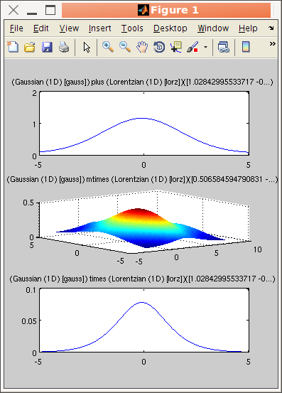 mrdivide(/) and
mpower(^) operator perform orthogonal axes multiplication,
with extension of the model dimensionality.
Examples are easier to understand, so let's see a few operations :
>> a = gauss  + lorz;		% addition
>> b = gauss  * lorz; 		% orthogonal axes multiplication 2x 1D -> 2D
>> c = gauss .* lorz; 		% parallel axes multiplication
>> c.Constraint = 'p(8) = 0;';	% avoid having two Background parameters
>> subplot([a b c])
In binary operations, passing one of the arguments as a string will simply insert the
corresponding code into the model Expression as the argument to the
operator. For instance the following statement appends a zero value
vector to the gauss model
value (axes are x,y,z,...
and parameters values are in p):
>> c = gauss + 'zeros(size(x))'
The addition operator plus (+)
used with a string argument which contains an equal sign '=' or ';' character
concatenates the string before/after the Expression of the model.
For instance the following example does the same as above,
explicitly setting the new signal value, and the next one displays a
text before evaluating the model :
>> c = gauss + 'signal = signal + zeros(size(x));';	% add code after the Expression (append)
>> c = 'disp(''Gaussian comming'');'+ gauss;		% add code before the Expression (prepend)
Last, when using a single word character string as one of the
arguments to a binary operation, a constant Parameter is used, for
instance :
>> c = gauss + 'Background'			% add a new Background parameter
>> c = gauss + constant('Background')		% same as above
>> c = gauss + constant				% same as above, but not naming explicitly the new Constant
>> d = gauss.*'Amplitude' + 'Background'	% add 2 new constant Parameters
You can also use the convolution related operators
- conv: convolution
- convn: normalized
convolution (which normalizes and centers the 2nd argument)
- xcorr: cross-correlation
In these methods, when one of the argument is scalar, a Gaussian
function of that width is built for convolution/correlation.
>> a = convn(lorz, 3)		% convolution of a Lorentzian with a Gaussian of width 3
>> a = convn(lorz, gauss)	% a Voigt function...
>> a = convn(lorz, 'double(b)'); a.Constraint = 'global b';	% convolute with a global variable 'b'
Methods generally mimic the Matlab default ones in functionality,
and are also similar to those of the iData
objects (see the Methods page).
It is possible to apply binary operators on mixed type arguments
(e.g. a Data set and a Model), in which case the result depends on
the arguments, as detailed in the 'binary operators with mixed
arguments' help.
Optimising
the iFunc model parameters
It is possible to optimize the model parameter values in order to
minimize or maximize the model value, with the 'fmin' method.
For this, any optimizer can be used, e.g.
>> p = fmin(model)
will use some guessed axes and automatic optimizer choice for the
optimisation. To start the optimization for a given initial
parameter set, use:
>> p = fmin(model, starting_pars)
The starting parameters can be given as a vector, structure or
string such as 'Intensity=1' as
explained above.
When given as a structure or a string, the resulting optimised
parameters are returned as a structure.
You may also set manually the optimizer configuration and axes to
use with:
>> p = fmin(model, starting_pars, options, x,y, ...)
Just as detailed in the Optimizers
documentation, you may specify the 'options' as the name of the
optimizer (then using its default configuration), a string, or a
structure, such as in the following examples:
>> p = fmin(model, starting_pars, 'fminpso')
>> p = fmin(model, starting_pars, 'optimizer=fminpso; OutputFcn=fminplot; Display=iter')
By default, the axes to use for the evaluation will be guessed. In
order to explicitly specify the axes to use, add them after the
options:
>> p = fmin(model, starting_pars, 'optimizer=fminpso; OutputFcn=fminplot; Display=iter', x,y, ...)
In all cases, it is strongly advised
to fix the non-relevant parameters, and bound the others, as
explained above.
For instance:
>> model= gauss1;
>> fix(model, 'all'); model.Intensity='free';
>> model.Intensity=1; model.HalfWidth=.5;
>> xlim(model, 'Intensity',[-2 2])
>> fmin(model)
ans =
   -2.0000         0    0.5000
>> fmin(model, 'Intensity=1')
ans =
    Intensity: -2
will search for the intensity that minimizes a Gaussian. This is of
course the lower Intensity bound, other parameters being fixed.
It is also possible to maximize the model parameters with the
similar 'fmax' method. The result is then the upper Intensity
bound.
>> model= gauss1;
>> fix(model, 'all'); model.Intensity='free';
>> model.Intensity=1; model.HalfWidth=.5;
>> xlim(model, 'Intensity',[-2 2])
>> fmax(model)
ans =
    1.9995         0    0.5000
Fitting model parameters onto data
NOTE: a more detailed documentation
on this topic is available in the Fit
page.
Once models have been assembled, it is possible to use them for
fitting, that is find the best parameter values to match a data set.
The syntax for this is :
>> p = fits(model, data, starting_parameters, options, constraints, ...)
The data can be given as an iData object,
a vector/matrix,
data=[
.... ]
a structure with members
data.Signal
data.Error
data.Monitor
data.Axes={x,y,...}
or a cell
data={
x,y, ... , Signal }
Similarly to the iData objects, the 'x'
1st rank axis corresponds to rows, 'y' to columns. When the data has
a higher dimensionality as the model, this latter is extended by
orthogonal multiplication to match the data dimensionality. It is
thus possible for instance to fit a 4D data set with the default
'gauss' model, which then results in the creation of the
'gauss*gauss*gauss*gauss' model.
The fit begins from the given starting values, or from guessed
values if entered as empty. Other options
and constraints, as well as
returned arguments, are the same as described in the Fit page. Empty input argument values request
the fit to use default values.
	>> data=load(iData, [ ifitpath 'Data/sv1850.scn' ])
	>> p=fits(data);	% fit to a gaussian
or with a specific optmiser choice:
>> [p,c,m,o]=fits(gauss,data,[],'optimizer=fminpowell; OutputFcn=fminplot');
The model value when the fit procedure ends is stored in the
output.modelValue member :
>> [parameters,criteria,message,output]= fits(model, data, initial_parameters,...)
which is an iData object when data is given as an iData. In
this case, fits(iFunc, iData,
...) is equivalent to fits(iData,
iFunc, ...), and you can directly plot the result on top of
the initial data with:
>> plot(data, output.modelValue)
When the data to be fitted is not an iData object, you can plot the
fit result from e.g.
>> plot(output.modelAxes,output.modelValue)	% 1D
>> surf(output.modelAxes{:},output.modelValue)	% 2D
E.
Farhi
- iFit/iFunc objects - Nov. 27, 2018 $Revision:1.7 $ - back to
Main iFit Page 

 Refer to the dedicated help on this topic in
the Models page, which also lists
pre-defined models (Gaussian, Lorentzian, exponential, lines,
quadratic, ...). Edit their code to see how to define new models:
 mrdivide(/) and
mpower(^) operator perform