iFit: plotting iData objects
Commands we use in this page:
plot, subplot, xlabel, xlim, title,
saveas,
methods
The
iData objects can be plotted. They
then show the
Signal, usually
divided
by the
Monitor, as a
function of the defined
Axes
(or default ones when not defined). A way to plot the raw
Signal is to set the
Monitor to 1 or 0.
You can of course display the object information with the disp
method:
>> a=load(iData, [ ifitpath 'Data/sv1850.scn' ])
>> disp(a)
or edit its values in a spreadsheet:
>> edit(a)
Plotting objects
in a single pane (plot)
The main plot method for iData objects is plot. It works for objects up
to ndims(a)<=3. Further
dimensionality objects may be visualized by means of projections and
slices, as seen below. The quantity which appears onto plots is the
Signal/Monitor. In order to
vizualize the raw Signal, set
Monitor to 1 with e.g.
>> a=load(iData, [ ifitpath 'Data/sv1850.scn' ])
>> plot(a)
>> old_mon=getalias(a,'Monitor');  % save the current Monitor alias if you wish to restore it afterwards
>> setalias(a,'Monitor',1);
>> figure; plot(a)
The plot windows offer 'camera ready' quality rendering using
openGL. Standard tools are available zoom, edit, pan, export image,
rotate, explore data points with a cursor, customize colors, ...
The plot style can be tuned to mesh, contour, line, scatter,
surface, volumes, waterfall, ...
Plots for 1D
objects
Let us import a simple 1D (vector Signal=f(x)
) data set into an iData object, and plot it:
>> a=load(iData, [ ifitpath 'Data/sv1850.scn' ])
>> plot(a);
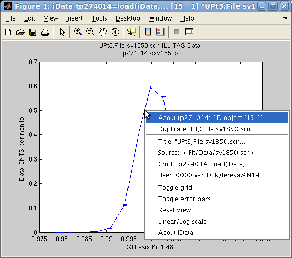
A standard Matlab figure appears, with the Signal and the Axis
of rank 1. The curve itself can be right-cliked in order to pop-up a
contextual menu which provides (see left image):
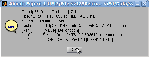
- an information dialog about the object (see right image above) and the
iFit/iData library version,
- the possibility to duplicate the view into an other window,
- simple ways to toggle a grid and error bar display,
- simple way to toggle linear or log scale for the Signal
- a 'Reset view' item
to re-plot the initial object view.
Tip: in case the contextual
menu item linear/log toggle does not satisfy your expectations, you
may try to directly plot the log of the object with (see Math operators)
>> plot( log10(a) );
As for any Matlab window, it may be edited using the arrow
tool  which allows to double-click the labels, title, the
axes and the curve in order to change e.g. the fonts, the text to
show, the colors.
The zoom tool  is also pretty useful
(hey ?). To revert to the full view, double click on the figure, or
select the contextual menu item 'Reset
view'.
The Matlab documentation about Graphics/Plots
and Plotting Tools/Figures, Plots, and Graphs provides a
full description of all the tools available in Matlab plot windows.
Most of the functionality can also be accessed from the Figure
menus. We encourage you to read all this, especially late at night
in winter.
Additional arguments can be given to plot in order to specify the line style and color, such as in
the standard Matlab plot
function, e.g. plot(a,'r--')
to draw a red dashed line. The special style 'hide_errorbars' will not show
error bars, but they can be made visible from the contextual menu.
The h=plot(...) function
returns a Matlab graphics handle (this is usually a number). It may
be used to perform further access and modification to the view.
Plots for 2D
objects
Similarly as for 1D objects, plots can be generated for 2D objects Signal=f(x,y), and show them up
as surfaces:
>> a=load(iData, [ ifitpath 'Data/ILL_D10.dat' ])
>> plot(a);
which results in a surface plot as shown aside.
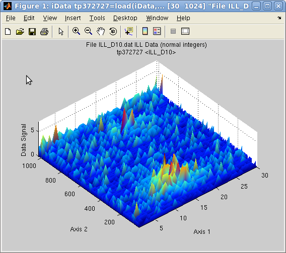 Plot 2D:
 plot(a) with
smooth view
Alternate rendering can be obtained with the plot options:
>> a=iData(peaks);
>> plot(a);           % a surface, same as surf(a)
>> plot(a,'mesh');    % a wired mesh, same as mesh(a)
>> plot(a,'contour'); % contour plot, same as contour(a)
>> plot(a,'contourf');% contour plot with filled regions, same as contourf(a)
>> plot(a,'surfc');   % a surface with contour plot below, same as surfc(a)
>> plot(a,'surfl');   % a surface with light, same as surfl(a)
>> plot(a,'plot3');   % a surface made of lines side by side, same as plot3(a)
>> plot(a,'scatter3');% a surface made of colored points, same as scatter3(a)
>> plot(a,'waterfall');% a surface made of colored points, same as waterfall(a)
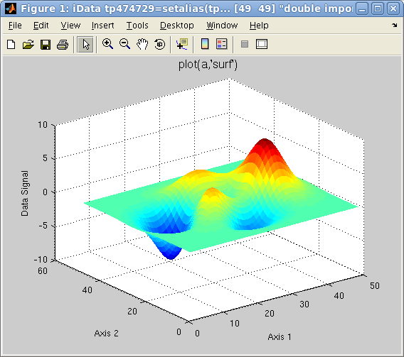
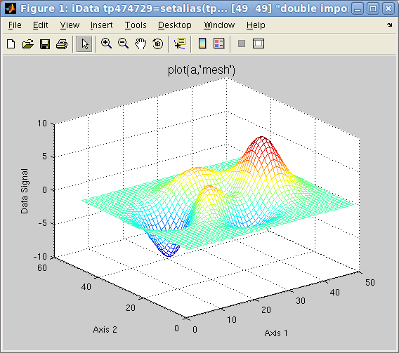
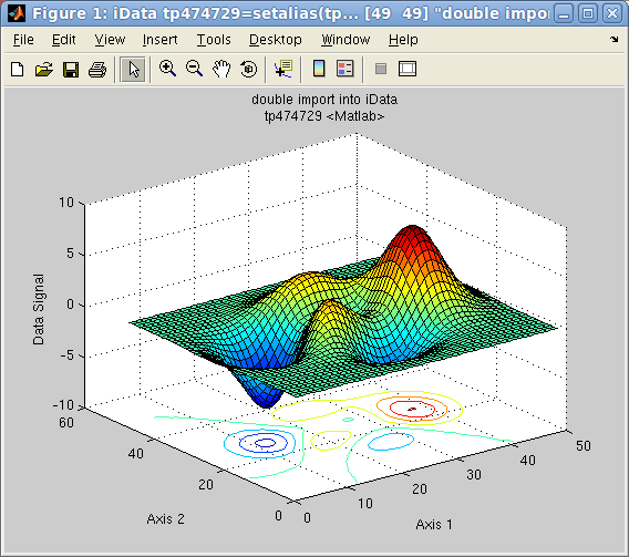 Plot 2D: left=plot
(a),
center=
mesh(a),
right=
surfc(a)
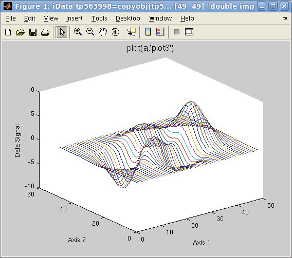
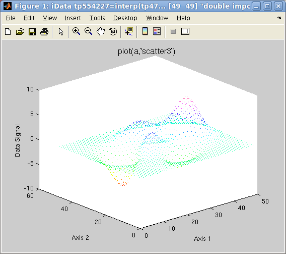 Plot 2D: left=plot3
(a),
right=
scatter3(a)
Other plot types can be requested with keywords in the second
argument to plot:
- contour3 (a countour in 3D)
- surfl (surface with light)
- pcolor (a flat matrix/image
view, may be advantageously coupled with the hide_axis option)
- stem3 (single points which
show elevation from basal plane)
Data shown as an
image (flat)
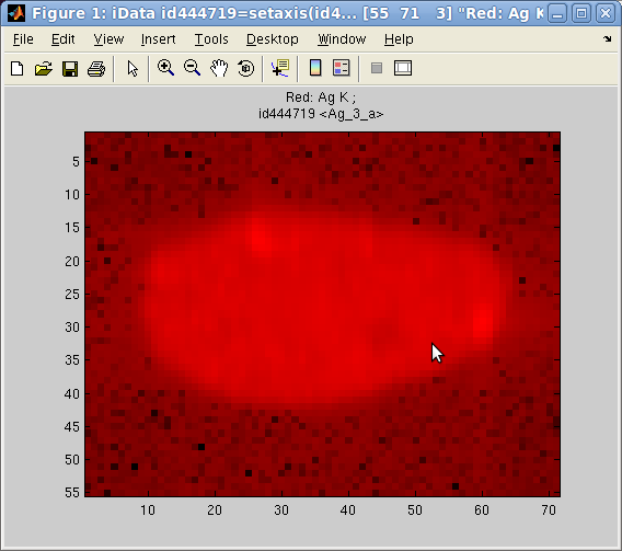 In
addition, the image(r,g,b)
plotting method allows to send up to 3 objects onto the RGB color
channels, and display them as a flat image (when using option='hide_axis') :
>> a = iData([ ifitpath 'Data/Ag_3_a.edf' ])
>> h = pcolor(a);			% full color image
>> h = image(log(a), 'hide_axes');	% red channel image
>> h = image([], a, 'hide_axes');	% green channel image
>> h = image([],[], a, 'hide_axes');	% blue channel image
Some of the RGB channels can be left empty to suppress one color.
Each object is re-scaled in the [0 1] range to use the full channel
colors. However, when using the option 'norm' keyword, the scaling is made global to
all images, enabling comparison of relative intensity between
channel contents.
An other possibility to supperpose different contributions with
separated colors is to use the colormap
method below.
Mapping an object
onto a surface (CData)
When a surface has been already plotted, either from the Matlab
standard surf or the iData plotting methods presented above, the
color shown on surfaces are usuyally the value of the data itself.
 It
is possible to map the values of any iData object onto a surface.
When the iData object does not match the surface dimensions, a
rescaling is automatically performed. This is achieved with the caxis method.
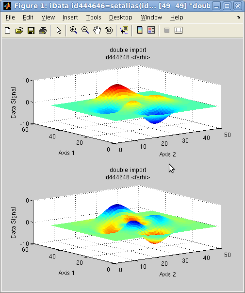
In the following example, we plot a surface, and then map the colors
shown on that surface (aka CData) with the Laplacian of the surface
(curvature):
>> a = iData(peaks);
>> h = subplot([ a a ]);
>> caxis(del2(a),h(2));	% we map the Laplacian onto the second plot
The initial object is shown in the upper panel, whereas the
re-mapped object is shown below. The blue regions indicate a
negative curvature (top of hills), and the red ones indicate a
positive curvature (bottom of hills).
Having separate
colors in plot of arrays
It is possible to associate one colormap (that is a set of colors
glued onto a surface) for each object displayed in a same coordinate
frame/window. The colormap function should then be used. It supports
the same options as plot, but colormaps can be specified in the list
of arguments. When ommitted, a set of predefined colormaps is chosen
for each object.
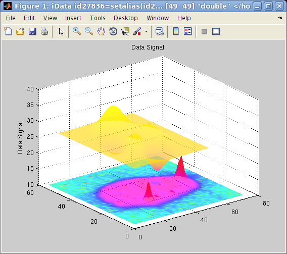
This plotting method is particularly pretty looking when using the 'shifted' option, which
then separate objects one from the other so that they can be well
identified on the figure. Choosing colormaps which are well
separated in color scales allow to visualize different
contributions, just like the image
plotting method.
>> a = iData([ ifitpath 'Data/Ag_3_a.edf' ]);
>> b = iData(peaks);
>> colormap(a/10000,hsv,b,spring,'shifted transparent interp');
The first object is set to scale, and plotted with the hsv color set. The second
object is shown with the spring color set. Adding the 'log' keyword to the
options will use the log of the signal for the color scale, in order
to enhance low signals.
Contextual menu
It is possible, by right-clicking on the surface or the axis lines,
to pop-up a contextual menu which provides the following operations:
- an information dialog about the object (see right image above) and the
iFit/iData library version,
- the possibility to duplicate the view into an other window,
- simple way to toggle a grid
- the possibility to smooth the surface appearance, add light
and make it semi-transparent. Consecutive light and transparency
selections enhance the rendering
- simple way to toggle linear or log scale for the Signal
- simple way to toggle a perspective rendering
- a 'Reset view' item
to re-plot the initial object view.
In addition to the edit  and zoom tools
  , a rotate view tool
  enables to change
the view-point.
NOTE: as
explained
in the iData axis definition,
the axis of rank 1 is usually assigned to the 'Y' label, and the
axis of rank 2 to 'X'.
Plots for 3D
objects
Objects that contain volumetric data Signal=f(x,y,z) can also be displayed as
iso-surfaces or semi-transparent volumes, such as in the following
example:
>> [x,y,z,v]=flow; c=iData(x,y,z,v); ;
>> plot(c);
The default plotting method used is an isosurface using an optimal
signal value. Other rendering can be plotted with e.g.:
>> plot(c,'surf median');    % plots the c=median(signal) isosurface, same as plot(d) [default]
>> plot(c,'surf mean');      % plots the c=mean(signal) isosurface
>> plot(c,'surf half');      % plots the c=(max-min)/2 isosurface
>> plot(c,'plot3');          % plots a volume rendering with semi-transparent style, same as plot3(c)
>> plot(c,'scatter3');       % a set of colored points in space, same as scatter3(c)
>> plot(c,'waterfall');      % a set of colored points in space, same as contourf(c) and waterfall(c)
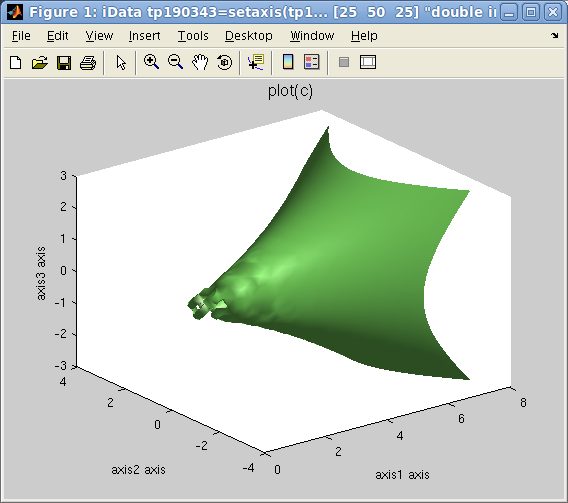
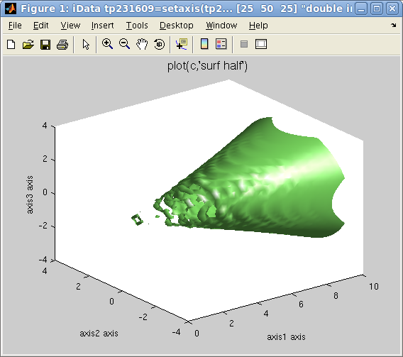 Plot 3D: left=plot
(d)
,
right=plot(d,
'surf half')
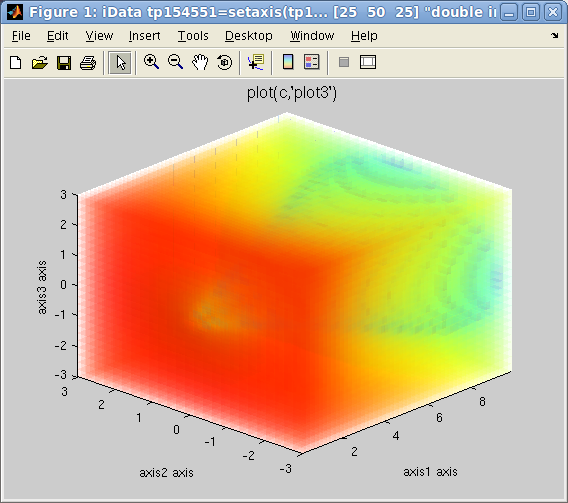
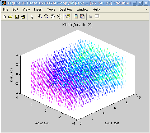
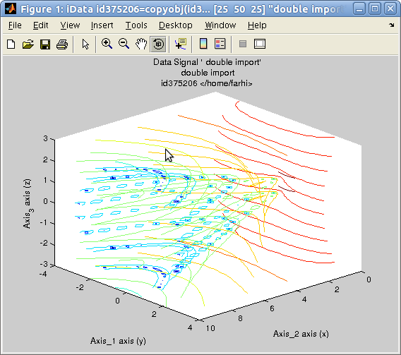 left=plot3
(d)
, center=scatter3(d),
right=waterfall(d)
It is possible, by right-clicking on the surface or the axis lines,
to pop-up a contextual menu which provides the following operations:
- an information dialog about the object (see right image above) and the
iFit/iData library version,
- the possibility to duplicate the view into an other window,
- simple way to toggle a grid
- the possibility to smooth the surface appearance, add light
and make it semi-transparent. Consecutive light and transparency
selections enhance the rendering
- simple way to toggle linear or log scale for the Signal
- simple way to toggle a perspective rendering
- a 'Reset view' item
to re-plot the initial object view.
In addition to the edit  and zoom tools
  , a rotate view tool
  enables to change
the view-point.
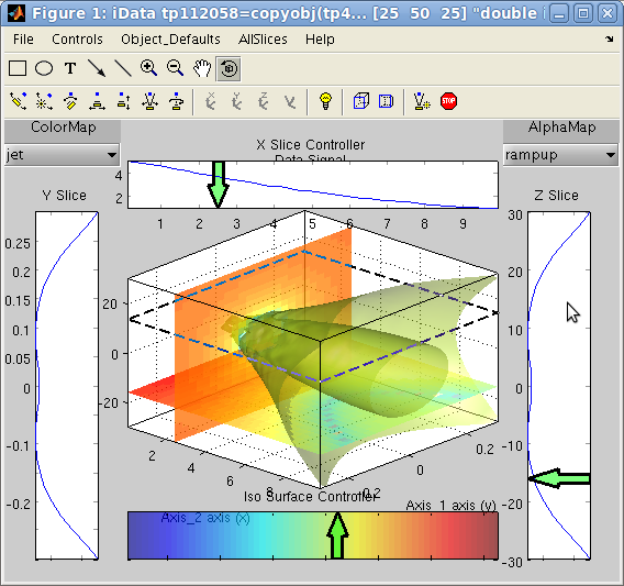
Last but not least the Slice-o-matic
viewer for 3D volumetric data set is requested upon command:
>> slice(c) % with ndims(c)=3
Slices and isosurfaces can be viewer with an interactive tool (see below).
NOTE: as
explained
in the iData axis definition,
the axis of rank 1 is usually assigned to the 'Y' label, and the
axis of rank 2 to 'X'.
Options for 2D and
3D objects
The 2D ans 3D rendering may be customized by mean of keywords added
to the second argument to the plot function call, as follows:
- flat, interp, faceted:
affects the type of shading used (see help shading).
- transparent, light:
adds transparency (see help
alpha), and add some light(see help light).
- clabel:
requests a labeling of contours, by value (see help clabel)
- axis tight, axis auto:
sets plot axis limits tight around the object, or automatically
optimized (see help axis)
- view2, view3:
displays 2D/3D views from top or oblique view
- painters
(bitmap drawing), zbuffer
(vectorial drawing): selects the Matlab painters for rendering.
- hide_axes hides
XYZ axes and labels, but retains the Title
- shifted for
overlayed plots makes sure plots are regularly shifted on the Z
axis for better shifted overlayed rendering.
A usage examples is
>> plot(a,'surf interp view2 axis tight transparent')
Plotting an object
array in a single plot
Overlayed plot
All plot functions can be overlay-ed with the usual hold on Matlab
command. However, the iData methods provide an integrated way to
plot an array of objects onto the same figure, such as in the
following example:
>> x=-pi:0.01:pi; a=iData(x,x);
>> a.Error=0;                         % replace default Error=sqrt(Signal) by no-error.
>> b=sin(a); c=cos(a); d=exp(-a.*a);  % create new objects by applying operator on the initial linear one
>> plot([a b c d]);                   % overlay all objects
This can also be applied to 2D and 3D objects, even though the
latter usually produces a crowded plot.
>> [x,y,z]=peaks; a=iData(x,y*10,z);
>> c=linspace(a,-a+50,10);            % continuously go from 'a' to a '-a+50' in 10 steps
>> plot(c);                           % plot all on the same figure
which overlays a set of objects, as shown below with a chosen view
angle.
![iData_plot_overlay: plot([array]) iData_plot_overlay: plot([array])](images/iData_plot_overlay.png)
![iData_plot_overlay_2D: plot([array]) iData_plot_overlay_2D: plot([array])](images/iData_plot_overlay_2D.png)
Plot overlay: plot([ array ]): left=1D,
right=2D
Any array of objects can be plotted, including object mix with
dimensionalities 1, 2 or 3.
Side by side
plotting: Single objects and Catenated objects (waterfall)
A common way to plot a set of 1D curves which depend on a
parameter is to plot them side by side (waterfall style), so as
to form a surface. Let us build an array of 1D objects and
assign it an additional axis.
>> x=-pi:0.01:pi; a=iData(x,x);
>> a.Error=0;                         % replace default Error=sqrt(Signal) by no-error.
>> b=sin(a); c=cos(a); d=exp(-a.*a);  % create new objects by applying operator on the initial linear one
The objects we have defined are 1D objects. In order to have
them appear in a 2D coordinate frame, one way is to simply
assign a new axis to each object, and then display them as a
surface:
>> a{2}=1; b{2}=1.5; c{2}=3; d{2}=5;  % assign a new 2D axis single value to each 1D objects
>> plot([a b c d],'surf');            % plot all as a set of lines side by side
>> waterfall([a b c d])               % same as above
>> surf([a b c d]
If the X axis (rank 2) has not been defined, the index of the
objects in the array is used. The surf method
'surf' and
'scatter3' methods are
here equivalen
t (colored
lines), whereas
'plot3'
and
'waterfall'
draw simple lines.
An other way to achieve a similar result is to assemble the 1D
objects into a 2D object, and then define the new axis values:
>> e=cat(2, [a b c d]);               % catenate 1D objects into a 2D object along 2nd axis
>> e{2} = [ 1 1.5 3 5 ];              % assign 2nd axis values in one go
>> plot(e,'mesh');                    % plot
which has the advantage that the new axis is directly assigned
to a vector, instead of independent single values.
![iData_plot_sidebyside: plot([ array_1D ], 'surf') iData_plot_sidebyside: plot([ array_1D ], 'surf')](images/iData_plot_sidebyside.png)
![iData_plot_sidebyside_cat:
plot(cat(2,[array]), 'mesh') iData_plot_sidebyside_cat: plot(cat(2,[array]),
'mesh')](images/iData_plot_sidebyside_cat.png) Plots side by side:
left=separated plots, right=catenated objects
Plots side by side:
left=separated plots, right=catenated objects
Plotting object
array in a set of panes (multiple-plots aka subplot)
![iData subplot([ array ]) iData subplot([ array
])](images/iData_subplot.png) In case one wishes to
display a number of objects into tiled independent coordinate
frames, all gathered into the same window, the subplot
function can be used the same way as with the overlay method shown above.
In case one wishes to
display a number of objects into tiled independent coordinate
frames, all gathered into the same window, the subplot
function can be used the same way as with the overlay method shown above.
>> x=-pi:0.01:pi; a=iData(x,x); a.Error=0; % replace default Error=sqrt(Signal) by no-error.
>> b=sin(a); c=cos(a); d=exp(-a.*a);       % create new objects by applying operator on the initial linear one
>> e=iData(flow); f=iData(peaks);          % create 2D and 3D objects
>> subplot([a b c d e f]);                 % plot all into a set of separate frames
The number of tiles is automatically set to a sensible arrangement
but can be set by hand by giving an additional [m n] vector of tile
dimensions.
>> subplot([a b c d e f], [ 2 3 ]);
Additional arguments can also be given to customize the type of plot
rendering:
>> subplot([a b c d e f], 'mesh tight');
>> subplot([a b c d e f], [2 3], 'surf light');
Plotting
projections and slices
Portions of an object can equally be displayed with plot and
subplot.
Plotting
projections
The integration operators sum,
camproj and trapz
can be used to produce data projections.
The sum computes the raw
serial sum of the signal along a given dimension. The trapz trapezoidal integration
computes the same, but takes additionally into account the axes
values. Finally, the camproj
does the same as sum, but on all other axes than the one specified.
In this respect, camproj
always produces a 1D vector which is the projection of the object on
the selected dimension.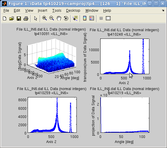 On a 2D
object sum(a,1) is the
same as camproj(a,2) and sum(a,2) is camproj(a,1).
>> a=iData([ ifitpath 'Data/ILL_IN6.dat' ]);	% import data
>> setalias(a, 'Angles', 'Data.FFFFFFFFFFFFFFFFFFFFFFFFFFFFFF_7(32:371)','Angle [deg]');
>> a{1} = 'Angles';	% define the angular axis
>> xlabel(a,'Time channel');
>> setalias(a, 'Wavelength','Data.FFFFFFFFFFFFFFFFFFFFFFFFFFFFF_10(21)','Neutron wavelength [Angs]');
>> setalias(a, 'ElasticChannel','Data.FFFFFFFFFFFFFFFFFFFFFFFFFFFFF_10(9)','Elastic channel position [ch]');
>> setalias(a, 'ChannelWidth','Data.FFFFFFFFFFFFFFFFFFFFFFFFFFFFF_10(18)','Channel time width [um]');
>> setalias(a, 'LSD','Data.FFFFFFFFFFFFFFFFFFFFFFFFFFFFF_10(27)','Sample-Detector Distance [m]');
>> subplot([ log(a) sum(a) trapz(a) camproj(a) ],'axis tight');
Plotting slices
Data slices and subsets can be obtained by selecting subspaces from
their corresponding indices.
>> a=iData([ ifitpath 'Data/ILL_IN6.dat' ]);
>> plot(a(:,622));                   % extract the object made from channel 622 on second axis, with all columns
The sliceomatic viewer is
displayed for 3D objects with
>> a=iData(flow);
>> slice(a)
You can then define the intensity level for the iso-surface, its
transparency, and create/move slices on 3 axes.
Setting plot
options: title, axes labels, axes limits
Even though it is possible to set the labels on a Matlab figure with
the title xlabel ylabel zlabel
functions, it is possible to store that information into the object,
so that further plots show it. It is also possible to extract
portions of an object by specifying the axes limits.
Setting labels,
title
To set the Signal label, use
>> title(a, 'a new Signal label')
which is different from the object title a.Title which holds the name of the whole data
set, independently of the assigned Signal in the Data. Also, the
object may be assigned a global label a.Label which may be used e.g. to store object
categories (background, calibration, with sample, ...).
The Signal label can be obtained with
>> title(a)
>> label(a,0)
>> label(a,'Signal')
Similarly, the axes can be assigned labels with
>> xlabel(a, 'a new X axis label');              % second axis (columns) ,or 1st axis for 1D objects
>> ylabel(a, 'a new Y axis label');              % first axis (rows)
>> zlabel(a, 'a new Z axis label');              % third axis
>> clabel(a, 'a new C axis label');              % fourth axis
>> label(a, rank, 'a new axis label for rank');  % any axis of given rank=1, 2, 3, ..., 0 for signal
All of these will be shown upon call to plot(a). The values can be obtained with e.g
>> xlabel(a)
>> label(a, rank)
>> ...
Setting axes
limits
It is possible to select a subregion of an object by specifying
limits among the axes. The resulting object does not hold the outer
limits data anymore.
>> xlim(a,[xmin xmax])
and similar functions ylim, zlim,
clim. Keep in mind that 'X' is along the second axis rank,
and 'Y' is along the first.
In order to only affect the view, we rather recommend to use the
standard Matlab commands xlim([xmin xmax]) and similar ylim, zlim and clim.
Exporting plots as figures and images
The figures can be exported from their File/Save as menu item. However, it is possible to
automate the export process by directly calling
>> saveas(a, filename, format)
where format may be jpg, png, pdf, HDF ... All formats are
detailed in the Save page.
The getframe method generates a snapshot picture
(thumbnail).
Importing plots as
iData objects
As seen in the Load documentation page, the
iData method can be used with graphical object including figure and
axis handle arguments.
>> a=iData(gcf);
E.
Farhi
- iFit/iData plotting - Aug. 22, 2017 1.10 - back to
Main iFit Page

 which allows to double-click the labels, title, the
axes and the curve in order to change e.g. the fonts, the text to
show, the colors.
  is also pretty useful
(hey ?). To revert to the full view, double click on the figure, or
select the contextual menu item 'Reset
view'.
 In
addition, the image(r,g,b)
plotting method allows to send up to 3 objects onto the RGB color
channels, and display them as a flat image (when using option='hide_axis') :
 It
is possible to map the values of any iData object onto a surface.
When the iData object does not match the surface dimensions, a
rescaling is automatically performed. This is achieved with the caxis method.
 and zoom tools
  , a rotate view tool
  enables to change
the view-point.


 and zoom tools
  , a rotate view tool
  enables to change
the view-point.
enables to change
the view-point.![iData subplot([ array ]) iData subplot([ array
])](images/iData_subplot.png) In case one wishes to
display a number of objects into tiled independent coordinate
frames, all gathered into the same window, the subplot
function can be used the same way as with the overlay method shown above.
In case one wishes to
display a number of objects into tiled independent coordinate
frames, all gathered into the same window, the subplot
function can be used the same way as with the overlay method shown above. On a 2D
object sum(a,1) is the
same as camproj(a,2) and sum(a,2) is camproj(a,1).