iFit: Mathematical operators
- A reminder on axes, monitors and
signal errors
- Unary operators
- Fourier transform
- Wavelet transform
- Derivatives
- Binary operators
- Convolution/correlation
- Comparisons
- Statistics, fitting and peak
searching, segmentation (k-means)
- Statistics
- Peak searching and model fitting
- Data segmentation
(partitioning/clustering, k-means)
- Projection, integration and sum
- Cutting, Merging and combining data
sets
- Cutting and selecting portions
of a data set
- The difference between addition
and combination
- Gluing an object content inside
an other one
- Appending and slicing data sets
- Creating arrays of objects
- Interpolation, smoothing,
intersection and union
- Intersection and union
- Interpolation
- Event data sets
- Re-binning and resizing
- Smoothing
- Manipulating object dimensions
Commands we use in this page:
iData, maths,
methods
In this documentation, we review most of the mathematical operations
that can be applied on iData objects. Separate help pages are
available for data import, export and fitting. A
full list is available in the methods
page.
A reminder on
axes, monitors and signal errors
The iData objects have been designed keeping in mind that any
measurement Signal is
recorded as a function of Axes
(e.g. time, energy, ...) and corresponds to a measurement quantity
(e.g. flux, integrated time for the measurement, ...), which we
label as a Monitor. In
addition, the Signal is attached to an uncertainty Error, which provides a
measurement of the accuracy of the Signal. You may get more details
about these definitions in the iData
object description page. Remember that axis of rank 1 is usually
associated to Y (vertical, along rows), whereas axis of rank 2 is
associated to X (horizontal, along columns) except for 1D object
where X is rank 1.
To get the signal and axes values, use:
>> a = iData([ ifitpath 'Data/ILL_IN6.dat' ]);
>> a{0}; % or getaxis(a, 0) to get the Signal (0-rank)
>> a{1}; % or getaxis(a, 1) to get the 1-st rank axis, that is 'x' for vector-type data, and 'y' for 2D+
>> a{2}; % or getaxis(a, 2) to get the 2-nd rank axis, that is 'x' for 2D+ data sets
In case the axis definitions is not what you want, you can re-assign
them using the setaxis
method (refer to the iData
object documentation).
The way all of these are used is listed below:
- All mathematical methods propagate
the Error
together with the Signal, assuming
Error distributions are Gaussian. The sections below detail the
way Errors are propagated.
- Binary operators use the Monitor
value to weight the respective ratio when performing the
operation. The Monitor
value is also affected by Mathematical operations that
renormalize the Signal. The
Monitor is usually a
value larger than 1. When
set to 0 (or empty), no weighting is used.
- The Axes are used in
binary operators to determine intersection of Signal ranges. A rebinning
of objects is automatically performed when the Axes sampling do not match.
Unary operators
All unary operators apply on a single object, element-by-element.
The Error for an operator
f is usually is
new
Error = Error.f'(Signal).
In the cases where the Error can not be determined analytically, and
approximation is obtained using
new
Error = f(Signal + ½Error) - f(Signal - ½Error).
Warning: all the
operators work on the normalised Signal/Monitor and Error/Monitor.
| Operator |
new Signal
|
new Error
|
new Monitor
|
Comments
|
abs
|
| Signal |
|
|
|
Absolute value
|
acos
|
cos-1(Signal)
|
Error/(√(1-Signal²))
|
|
Arc cosine. Signal should be
[-1:1]
|
asin
|
sin-1(Signal)
|
Error/(√(1-Signal²)) |
|
Arc sine. Signal should be
[-1:1] |
atan
|
tan-1(Signal)
|
Error/(1+Signal²) |
|
Arc tangent.
|
cos
|
cos(Signal)
|
-Error*sin(Signal)
|
|
Cosine. Signal is in [rad]
|
sin
|
sin(Signal)
|
Error*cos(Signal)
|
|
Sine. Signal is in [rad] |
tan
|
tan(Signal)
|
Error/cos²(Signal)
|
|
Tangent. Signal is in [rad] |
cosh, sinh, tanh
|
|
|
|
Hyperbolic trigonometric
functions
|
| acosh, asinh, atanh |
|
|
|
Inverse hyperbolic
trigonometric functions |
exp
|
eSignal
|
Error*eSignal |
|
Exponential
|
log
|
ln(Signal)
|
Error/Signal
|
|
Logarithm (Neperian, base 2)
|
log10
|
log10(Signal)
|
Error/(ln(10)*Signal)
|
|
Logarithm (base 10) |
sqrt
|
√Signal |
Error/(2√Signal) |
√Monitor |
Square root
|
ctranspose and
'
|
Signal'
|
Error'
|
Monitor' |
Complex conjugate transpose
|
transpose and
.'
|
Signal.'
|
Error'
|
Monitor'
|
Non conjugate transpose.
|
permute
|
permute(Signal)
|
permute(Error) |
permute(Monitor) |
dimensionality permutation
(generalized transposition)
|
floor
|
floor(Signal)
|
floor(Error)
|
|
Round towards -∞ Make it
integer.
|
| ceil |
ceil(Signal)
|
ceil(Error)
|
|
Round towards +∞ Make it
integer. |
round
|
round(Signal)
|
round(Error)
|
|
Round towards nearest
integer.
|
sign
|
sign(Signal)
|
0
|
|
Sign of Signal elements.
|
uminus and
-
|
-Signal
|
|
|
Opposite
|
imag
|
ℑ(Signal)
|
|
|
Imaginary part
|
real
|
ℜ(Signal)
|
|
|
Real part
|
fft
|
FFT(Signal)
|
FFT(Error)
|
|
Fourier
transform (see below)
|
| ifft |
FFT-1(Signal) |
FFT-1(Error) |
|
inverse Fourier transform |
cwt
|
Wavelet(Signal)
|
|
|
Continuous
wavelet transform (see below)
|
del2
|
∇2(Signal)
|
∇2(Error) |
|
Laplacian
∑i ∂2Signal/∂2Xi |
gradient
|
∇(Signal)
|
∇(Error) |
|
Gradient
(partial derivatives). See also the 'jacobian'
operator for coordinate changes.
|
diff
|
∇1(Signal) |
∇1(Error) |
|
Gradient on 1st axis (rows)
|
sum
|
∑(Signal) |
√∑(Error²) |
|
Sum of the Signal elements
(see below)
|
prod
|
∏(Signal) |
∏(Signal+Error/2)-∏(Signal-Error/2) |
|
Product of the Signal
elements |
trapz
|
∫(Signal) |
√∫(Error²) |
|
Trapezoidal integration
|
cumsum
|
∫0x(Signal) |
√∫0x(Error²)
|
|
Primitive
|
smooth
|
Smoothed(Signal)
|
Smoothed(Error) |
|
Robust spline smoothing based
on cosine transform
|
kmeans
|
Partition indices
|
0
|
|
Data
segmentation (k-means)
|
pca
|
Principal component
coordinates
|
0
|
|
Principal
component analysis
|
resize
|
Resized signal
|
resized Error
|
resized Monitor
|
fast resize with
interpolation
|
reducevolume
|
smaller Signal
|
-
|
-
|
data set reduction
|
sort
|
sorted Signal
|
-
|
-
|
sorted data set along a
dimension
|
Here is an example using unary operators:
>> a = iData([ ifitpath 'Data/ILL_IN6.dat' ]);
>> b = [ log(a) floor(a) sqrt(a) ]
b =  array [1  3] iData object:

Index     [Tag]     [Dimension]                           [Title] [Last command]          [Label]
    1  tp362134     [340  1024] 'File ILL_IN6.dat ILL Data (n...' tp362134=log(tp36213...
    2  tp362140     [340  1024] 'File ILL_IN6.dat ILL Data (n...' tp362140=floor(tp362...
    3  tp362145     [340  1024] 'File ILL_IN6.dat ILL Data (n...' tp362145=sqrt(tp3621...
The 1/Signal is obtained
with the binary operator division.
The sqr operator is a short
cut for power 2.
Fourier transform
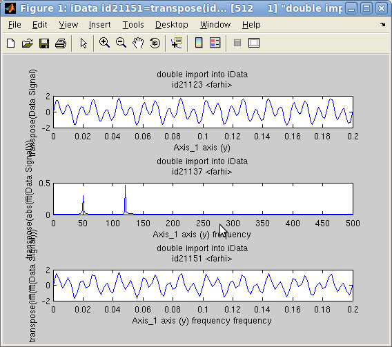 The Fourier
Transform operators fft
and 'inverse' ifft perform
a Discrete FFT computation from an N-dimensional object. The axes
are converted to frequency/reciprocal axes.
In the following example, we create an object which Signal is the
sum of 2 sine functions with frequencies 50 and 120 Hz. Then we
compute its FFT, and again its inverse FFT.
>> t=linspace(0,1,1000);
>> a = iData(t,0.7*sin(2*pi*50*t)+sin(2*pi*120*t)+0.05*randn(size(t)));
>> c=fft(a); d=ifft(c); subplot([ a abs(c) d ]);
The plot on the side shows that the two sine components are
identified (the FFT is shown in modulus), and the FFT-1(FFT)
is indeed the initial signal (within the computation
approximations).
The convolution operator, which uses FFT multiplication, is detailed
below. The frequency power-spectrum is
the square of the modulus of the FFT, sqr(abs(FFT)).
Wavelet transform
Going further than the FFT, the cwt
method computes the continuous
wavelet transform of a data set. It corresponds to the
decomposition of the signal along a wavelet basis function set, that
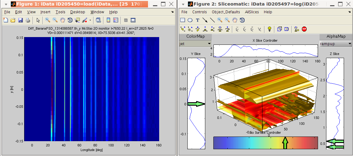
is a multi-scale analysis of the signal along an axis. In the
following example, we analyse a 2D powder neutron diffractogram with
the cwt and the slice methods.
>> a=iData([ ifitpath 'Data/Diff_BananaPSD_1314088587.th_y');
>> w=cwt(a, 2);	% the cwt along the axis rank 2 (scattering angle)
>> plot(a); slice(log(abs(w).^2))	% plot the initial data set and its cwt power spectrum
The resulting plot shows the sharp features (peaks) for small
'periods', and the broad features (background) for large periods.
The period axis is here shown in log10 scale of the initial axis
(degrees) and corresponds to the width of the wavelet.
Reference: Grinsted,
A., Moore, J.C., Jevrejeva, S. (2004) Application of the cross
wavelet transform and wavelet coherence to geophysical time series,
Nonlin. Processes Geophys.,
11, 561–566,
doi:10.5194/npg-11-561-2004.
Derivatives and
variable change (Jacobian)
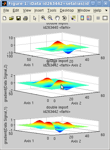 The gradient
operator computes the partial derivatives
∇ of an object. (see Gradient definition)
∇a = (∂a/∂Y ∂a/∂X
∂a/∂Z ...)
The resulting objects are sorted by axis rank, that is partial(X) is
2nd, partial(Y) is 1st, partial(Z) is 3rd, etc. In case the axis
sampling/binning is not regular, a re-binning is automatically
performed. For 1D objects, the gradient is the derivative. In the
following example, we compute the 2D gradient of an object, and plot
them.
>> a=iData(peaks);
>> g=gradient(a); subplot([ a g(1) g(2) ]);
The diff method computes
the gradient for the rows only (1st axis).
The del2 operator computes
the Laplacian Δ=∇2 of an object (see Laplacian definition)
∇2a = ∑i (∂2a/∂Xi2)
which is a measure of the curvature
of the object. In this sense, for an N dimension object, it
schematically returns, with the del2
standard Matlab function, 2N*del2(Signal).
In
case the axis sampling/binning is not regular, a rebinning is
automatically performed.
Finally the jacobian
operator (see Jacobian
definition) enables to perform a variable change in the
representation of the Signal. This corresponds to a new axis
definition with consecutive correction of the Signal so that the
integral value is retained between the different space
representations.
Suppose we want to perform a coordinate change from the axis system
X={X1, ... Xn} to a new
space Y={Y1, ...Yn} where
n is the dimensionality of
the object a Signal. Then
the Jacobian of the object is:
J(a,
X,
Y) = [ dYi/dXi ]ij
The new object b
infinitesimal element (pixel/bin) in the new representation which
ensures ∫ a dX = ∫ b dY is such that:
b
=
a | dY/dX |
which requires to estimate the Jacobian determinant for each
pixel/bin in the initial object a.
As the Signal holds a single scalar value in each bin, J is the division of the
gradient of Y over the
gradient of X for the
whole Signal.
Binary operators
The binary operators take two objects, and perform a relational
operator, element-by-element. In the following we use the notations:
- s1, e1 and m1 are the Signal,
Error and Monitor
of the 1st object, resp.
- s2, e2 and m2 are the Signal,
Error and Monitor
of the 2nd object, resp.
- s3, e3 and m3 are the Signal,
Error and Monitor
of the resulting object, resp.
When not defined, the Monitor
is set to 1, and the Error
is set to √Signal. When the
Monitor is set to 0, the Signal is not divided by it. Then the
binary operator result has the other object's Monitor (which may
also be 0).
Operator
|
Signal (s3)
|
Error (e3)
|
Monitor (m3)
|
Description
|
plus and
+
|
m3*(s1/m1+s2/m2)
|
√[(e1/m1)²+(e2/m2)²]
|
m1+m2
|
addition
|
minus and
-
|
m3*(s1/m1 - s2/m2) |
√[(e1/m1)²+(e2/m2)²] |
m1+m2 |
subtraction
|
times and
.*
|
s1 * s2 |
s3*[(e1/s1)²+(e2/s2)²] |
m1*m2
|
multiplication (element by element).
When object orientations are complementary (orthogonal), the
final object is built with dimensionality expansion.
|
| mtimes and * |
s1 x s2
|
e1 x e2
|
m1 x m2
|
matrix multiplication
|
rdivide and
./
|
m2²*(s1/s2) |
s3*[(e1/s1)²+(e2/s2)²] |
m1*m2 |
division (element by element).
When object orientations are complementary (orthogonal), the
final object is built with dimensionality expansion. |
| mrdivide and / |
see above
|
see above |
see above |
matrix division: currently
equivalent to the divide
operator
|
combine and
\
|
s1+s2
|
√[e1²+e2²] |
m1+m2
|
add Signals and Monitors
independently (see below).
Event lists objects are catenated.
|
power and .^
|
m3*(s1/m1)(s2/m2)
|
s3*[s2*e1/s1+e2*ln(s1)]
|
m1m2
|
exponentiation. When object
orientations are complementary (orthogonal), the final
object is built with dimensionality expansion.
|
comparisons: lt, le, gt, ge, ne, eq
|
comparison(s1, s2)
|
√[(e1/m1)²+(e2/m2)²]/[s1/m1+s2/m2] |
1
|
binary comparisons
|
conv
|
FFT-1(FFT(s1)*FFT(s2))
|
s3*[(e1/s1)²+(e2/s2)²] (this may be inappropriate) |
m1*m2
|
convolution
(see below)
|
deconv
|
|
|
|
iterative deconvolution (see below) |
xcorr
|
FFT-1(FFT(s1)*FFT*(s2)) |
s3*[(e1/s1)²+(e2/s2)²] (this may be inappropriate) |
m1*m2 |
cross
correlation (see below) |
interp
|
s1 onto s2
axes
|
e1 onto s2
axes
|
m1 onto s2
axes
|
interpolation (linear is
default, see below)
|
corrcoef
|
cov(s1,s2)/σ(s1)σ(s2) in
[-1:1]
|
|
|
Pearson
correlation coefficient
|
All these operations find intersection ∩ between objects (when axes
are e.g. partly
overlapping), rebin objects when axes have a different sampling, and
then perform the mathematical operation. In case some objects have a
lower dimensionality, they are extended along missing dimensions (by
mere duplication) to match the higher dimensionality, so that the
operation can be performed.
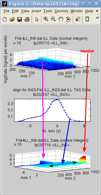 The following
example adds a 2D data set with a 1D data set, which is extended.
The intersection selects only the positive axis values from the 1D
object, here in [0 5]. As the 2D object has no default Monitor (set
to 1), we set it to 1/10 of the corresponding mean value in the 1D
object (if not done so the IN6 data is under weighted compared with
the IN20 data for which Monitor is high). The magenta and blue
arrows indicate how the data is added, and the 1D data set extended
along the Axis 2. as shown
with the double arrow.
>> a = iData([ ifitpath 'Data/ILL_IN6.dat' ]);
>> b = iData([ ifitpath 'Data/ILL_IN20.dat' ]);
>> set(a,'Monitor', mean(b.Monitor)/10);
>> c = a+b;
>> subplot([ log(a) b log(c) ] ,'tight')
Warning: It
is
important
to
check
that
the
axes
and
Monitor
values
are
consistent
when
performing
binary
operations,
otherwise
the
intersection
may be empty, or the corresponding Signal weighting may be wrong.
The combine operation will
be detailed in the section 'Merging and
combining data sets' below. In particular, the difference
between the summation and the combination will be detailed there.
All binary operators can also be used between one iData object and a
file name, in which case the corresponding data file is first
imported before the operation is performed.
>> a = iData([ ifitpath 'Data/ILL_IN6.dat' ]);
>> c = a+[ ifitpath 'Data/ILL_IN20.dat' ];
Convolution/correlation
The convolution
operator conv uses a FFT
method to compute the convolution of one iData with anything else.
In the background it uses the fconv and fconvn function (see Models), which can be called
directly when building fit functions.
The convolution operator can be given additional options in order to
control the accuracy and the size of the returned object
>> c = conv(a,b);		% returned convoluted object with size which is size(a)+size(b)+1
>> c = conv(a,b, 'same');	% returned convoluted object with size which is size(a)
>> c = conv(a,b, 'valid');	% returned convoluted object with size which is size(a)-size(b)+1
>> c = conv(a,b, 'pad');	% pads 'a' with starting/ending values to minimize border effects
>> c = conv(a,b, 'center');	% centers 'b' so that convolution does not shift 'a' axes
>> c = conv(a,b, 'norm');	% normalizes 'b' so that convolution does not change 'a' integral
>> c = conv(a,b, 'background');	% subtracts minimal value in 'b' so that convolution does not change 'a' integral
>> c = conv(a,b, 'deconv');	% deconvolution, but very sensitive to noise (use with caution)
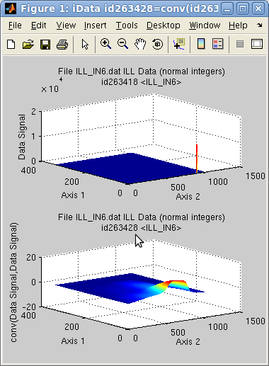 When the 1st object has to be convoluted with
a response function (e.g.
instrument resolution function), the usual options to use should be:
>> c = conv(a,b, 'same pad background center norm');
>> c = convn(a,b);	% same as above in a shorter call
To perform an auto-convolution, just use:
>> a = iData([ ifitpath 'Data/ILL_IN6.dat' ]);
>> c = convn(a,a);
When the second argument 'b' is given as a scalar, a Gaussian with
that width is built.
>> c = convn(a, 3) % convolution of an iData with a normalized Gaussian of width 3
This is very useful when a measurement has to be corrected with the
response of the probe (instrument). In this case, a fit of the data
may be carried out as:
>> global b;			% holds the convolution function as a single vector/matrix or iData object
>> h = convn(gauss, 'double(b)');	% creates a fit function with convolution
>> h.Constraint= 'global b'; 	% declares b as an external global variable
>> p = fits(a, h);
where the vector/matrix 'b'
holds the response function (filter) with the same axis binning as the object 'a'. A way to force the right
binning is to use:
>> c = interp(b, a);
if the axes of 'b' match
the ones from 'a' in range
(overlap).
An other example of fit function with convolution is detailed in the
Models help page.
The deconv operator performs a deconvolution, using either
FFT's or with an iterative method.
Similarly, the xcorr
operator computes the cross
correlation of two signals. The auto-correlation is simply xcorr(a).
Last, the corrcoef method
returns the Pearson
product-moment correlation coefficient, which measures the
similarity between two data sets (1=equal, 0=non correlated,
-1=anti-correlated).
Warning: The accuracy
of the conv and xcorr operators depends on the
axis sampling. A coarse axis sampling (that is a reduced number of
points under a peak, e.g. less than 5) must be avoided. A rebinning
of the objects using e.g. interp(objects,
5) may solve such issue.
Comparisons
The usual comparison binary operators
- greater: gt >
- greater or equal: ge >=
- lower: lt <
- lower or equal: le <=
- equal: eq ==
- not equal: ne ~=
are also implemented. They compares the Signals, taking the Monitor
weighting into account. The associated error bar is normalized to
the mean signal.
Statistics, fitting and peak
searching, segmentation (k-means)
A few methods have been written to analyze the Signal from objects.
This includes peak searching, first and second moment distributions,
and model fitting.
Statistics
The usual min, max, mean,
and median methods can be
applied onto iData objects, and return the corresponding statistics
for the Signal. The operation is performed for one given
axis/dimension, e.g. along y, x, z ...
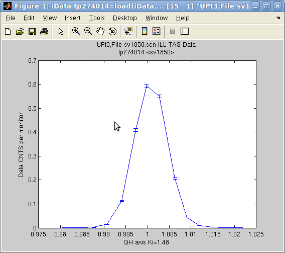
The std method provides an
easy way to determine Gaussian widths of Signal distributions along
axes. It returns the half width (2nd moment) and center (1st moment)
of the Signal distribution.
>> a = iData([ ifitpath 'Data/sv1850.scn' ]);
>> [w,x]=std(a)
w =
    0.0036
x =
    1.0007
>> [ min(a) max(a) median(a) mean(a) ]
ans =

            0         7387          119       1630.7
indicates that the Signal
is distributed in 1.0007 ± 0.0036, and gives min, max, ... As a
comparison, the fit to a Gaussian function returns
>> fits(a)
   'Amplitude'    'Centre'    'HalfWidth'    'Background'
      0.67857       1.0008    0.0034641   0.00024067
which is about the same as the 1st and 2nd moment estimates. Here,
the Amplitude fit
parameter is the one for Signal/Monitor,
which is indeed different from the value returned by max when Monitor is not 1. Use setalias(object, 'Monitor',1)
to get similar values from fits
and max in this example.
Note: If you get an
imaginary width from std
you may use a negative dimension specification, e.g. std(a, -1), in order to
subtract automatically the minimum value from the object, and get a
better estimate.
To get the width and centroid of a multi-dimensional
object, you can use an array of dimension specification, e.g.:
>> a = iData(peaks);
>> [w, x] = std(a, -(1:ndims(a))); % we subtract the minimum value (negative dimension spec.)
It is also possible to compute with the corrcoef method the
correlation coefficient between an object and something else, e.g. a
vector, an iFunc model or a single vector
of same length as the object signal.
These operators apply iteratively on object arrays. The mean and median then point to the combine operator, the min and max return the minimum and
maximum along all objects.
Peak searching
and model fitting
The peaks method makes an
automatic analysis of a vectorial Signal (that is projected along
one given dimension) of an object, and determines the underlying
baseline (background), apparent peak position and width, based on a
shifting Gaussian estimate [see Slavic, Nucl. Inst. Meth. 112 (1973) 253 ; M. Morhac, Nucl. Inst. Meth. A 600 (2009) 478].
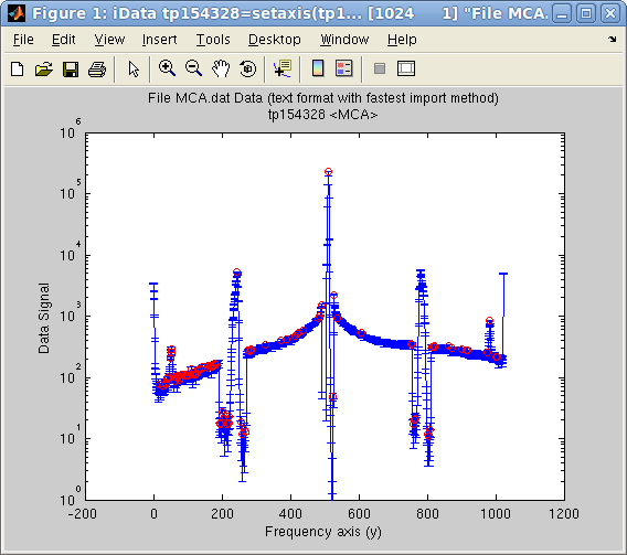 This
method works remarkably for signals with sharp peaks. The following
example displays the automatically found peaks on top of the object
view:
>> a = iData([ ifitpath 'Data/MCA.dat' ]);
>> setalias(a,'Signal','Data.Counts(:,2)');
>> [half_width, center, amplitude, baseline]=peaks(a);
>> plot(a); hold on;
>> plot(center,amplitude,'ro'); set(gca, 'yscale', 'log')
The first dimension (projection along rows, rank 1) is selected by
default for the analysis, but it may be specified as the second
argument. For broader peaks, a 3rd argument can be used to specify
the length m of the moving
window used for the analysis, which should typically be about the
number of point forming a peak (default is about 5).
As opposed to the std
method shown above, which only provides one Gaussian estimate, the peaks method can handle as many
peaks as necessary, and is very fast. It also works with iData
object arrays. This method is also used as a basis to determine some
starting parameters for most fit functions (see the Fitting and the Optimizers
pages).
In the case where a better peak estimate is required, or any other
advanced model parameter determination, the fits method can be used.
This latter makes use of the eval
method, which evaluates a model function onto the object axes.
Data segmentation
(partitioning/clustering, k-means)
It is possible to perform a statistical analysis of a data set in
order to classify it into a number of categories. This is called
segmentation, and a usual method to achieve it is the k-means
algorithm. The corresponding iData method is kmeans :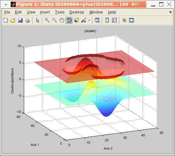
>> a = iData(peaks);
>> b = kmeans(a, 3);	% request segmentation in 3 groups
>> plot(a, b+5);	% overlay data set and segmentation result
The wavelet transform cwt
may also be used to perform a peak analysis, separating sharp
features from broad ones (see above).
The principal
component analysis (PCA) methodology consists in finding
similarities between data sets. Groups of 'close' data sets can then
be defined. The corresponding iData method is pca .
Projection, integration and sum
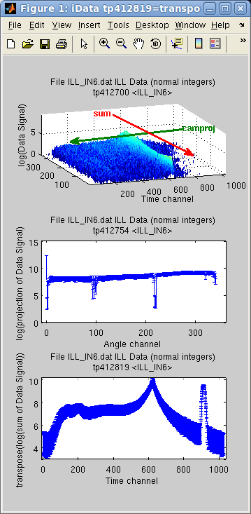 There are a
number of methods used to extract projected and summed objects.
Technically, the projection on one axis is the sum along all other
axis.
sum(a, rank) = ∑ Signal(rank axis index)
camproj(a, rank) =
∑ Signal(all axes except
rank)
In the following example, the imported object is assigned two axes,
and we then display the difference between the sum and the projection with camproj, onto the 1st axis (y).
Of course this can be changed by specifying explicitly the desired
axis rank used for operation as the second argument.
>> a = iData([ ifitpath 'Data/ILL_IN6.dat' ]);
>> xlabel(a, 'Time channel'); % 2nd axis
>> ylabel(a, 'Angle channel');% 1st axis
>> subplot([ log(a) log(camproj(a)) log(sum(a)) ],'tight');
The camproj method always
returns a 1D result (or a single value). The sum reduces the dimensionality
of the object by the number of axes summed. Similarly, the prod
method compute the multiplication along a given axis:
prod(a, rank) = ∏ Signal(rank axis index)
The summation with the sum
method does not take into account the axes values. In the case a
proper integration is needed, the trapz
method can be used for integration using the trapezoidal
approximation on the axis values and step dx
trapz(a) = ∫ Signal(rank
axis) dx
 which will reduce the dimensionality, and be
roughly equivalent to sum
when dx=1.
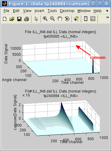
Last, the accumulated
versions of sum, trapz and prod,
cumsum, cumtrapz
and cumprod, return
objects of same dimensionality for which the operation is performed
gradually along the chosen axis. The last slice along the axis
contains the sum and prod results.
In the following example, the sum along the first dimension (y=Angle
channel) reveals that an intense peak exists in first angle channel,
resulting in a constant line (right side of the sum), whereas the
elastic line, is gradually summed over all angle channels, showing
inelastic contribution on its shoulders.
>> subplot([ (a) cumsum(a) ] ,'tight')
The cumtrapz is the primitive
of the Signal, which is
equal to cumsum when the
axis step is dx=1.
The norm method computes
the norm-2 of the object Signal,
that is
norm(a) = ½ ∑ |Signal|²
The camproj can also be
used with dim='radial' in
order to integrate a data set radially. This integration can also be
coupled with a more general Cartesian to spherical coordinate
transformation with cart2sph
: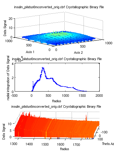
>> a = iData([ ifitpath 'Data/*.cbf' ]);
>> b = camproj(a,'radial'); % returns a distribution to be transformed into an histogram
>> c = cart2sph(a);
>> subplot(log(a), hist(b,500), log(c))
To efficiently and quickly reduce the dimensionality of an object,
we also recommend the resize
method by specifying a singleton dimension:
>> b = iData(flow);		% is 3D
>> resize(b, [25 50 1]);	% makes a 2D object from a 3D one
Then use squeeze(b) to
remove any remaining singleton dimension.
Cutting, Merging
and combining data sets
Cutting and
selecting portions of a data set
A way to select a subset of an object from its axis rang is to use xlim, ylim, zlim, clim for
respectively 2nd (X is 1st for 1D objects), 1st, 3rd and 4th
dimensions. It is also possible to directly use find:
>> a = iData([ ifitpath 'Data/ILL_IN6.dat' ]);
>> b = xlim(a, [100 200]);					% selects the object with X axis ranging from 100 to 200
>> b = a(:, find(  100 <= a{2} & a{2} <= 200 ));				% same as above: X is rank 2(columns)
>> c = a(find(50 <= a{1} & a{1} <= 150),find(100 <= a{2} & a{2} <= 200));	% cuts along X(rank2) and Y axes(rank1, rows)
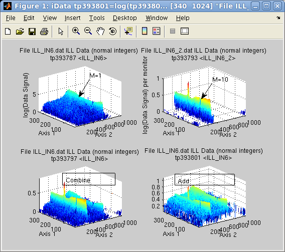
The difference between addition and
combination
The combine operation
performs an addition of the Signal
and the Monitor. This is
of great use when merging results from similar experiments, possibly
performed in slightly different configurations (e.g. counting time, statistics,
...). This means that combining two data sets is usually more
complex than just adding the two Signals,
especially when axes are not exactly the same and Monitors are not equivalent.
Suppose we perform a measurement providing a Signal S1 for a given
acquisition time M1 (Monitor). The data to be used
in mathematical operations is S1/M1.
Then we repeat that same measurement, providing Signal S2 and Monitor M2. If, for this
example, S2 and M2 are similar to S1 and M1, then the combination of the
two data sets should produce a similar signal as any of the two
measurements, but with better statistics. But the addition should
produce about twice any of the measurements. In short the rules for
the operations are:
- combination: (S1+S2) over monitor (M1+M2)
- addition (sum): (M1+M2)*(S1/M1+S2/M2) over monitor(M1+M2)
as listed in the binary operators
Table. The addition
performs the operation per
Monitor value (weighted), whereas the combine operation adds raw Signals and Monitors (unweighted). Changing
the Monitor of the objects
affects the relative weight used for the summation during the
addition operation, but not the combine operation.
When one of the Monitors is set to 0, the Signal is left as
is. In the case where the two objects have a 0 Monitor, the addition
results simply in the sum of the Signals.
Suppose the first object is the result of a measurement during 1
minute (liquid, M1=1), whereas the second lasted 10 minutes. This
means that per Monitor
value, the second signal (Vanadium,, M2=10) is much lower than the
first one (see upper right signal in subplot aside, compared with upper left) but has a
stronger statistical weight.
>> a = iData([ ifitpath 'Data/ILL_IN6*.dat' ]);
>> a(1)=setalias(a(1),'Monitor', 1);
>> a(2)=setalias(a(2),'Monitor', 10);
>> b=combine(a)             % combine/merge
>> c=a(1)+a(2);             % addition
>> subplot([ log(a) log(b) log(c) ], 'tight');
The combined Monitor is
M=11, which means that the first data set will appear much lower
than initially (the initial Monitor was M1=1) in the combined data
set. However, for the add operation, it appears much higher, as each
Signal/Monitor is added
separately.
The '\' operator is used as
a shortcut for combine, so
that combine(a,b) is the
same as a\b.
Gluing an object
content inside an other one
As a complement to addition and merging, it is also possible to glue
an object 'a' content inside an other one 'b'. In this case, the
overlapping region from 'b' is fully replaced by the corresponding
one in 'a', without addition/merge. The syntax is
>> b(1) = a;
Appending and
slicing data sets
An other way to make use of a set of data from a series of
acquisitions is to append them one after the other. This operation,
also referred as concatenation,
may be performed along an existing dimension (one after the other),
or along a new dimension (side by side), which then increases the
object dimensionality. The operator used here is cat.
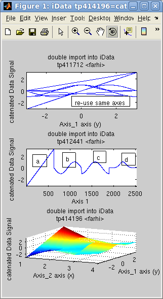 In the following example, the object d is the concatenation of 4
objects [a b c d],
sequentially. The concatenation of the 4 axes in 'd' is the repetition of the
initial axis. We then create an 'f'
object for which the axis is reset to the default, showing indeed
the concatenation of objects. Last, we assemble the same data set
side by side onto a new dimension, creating a surface 'g'.
>> x=-pi:0.01:pi; a=iData(x,x);
>> a.Error=0;                         % replace default Error=sqrt(Signal) by no-error.
>> b=sin(a); c=cos(a); d=exp(-a.*a);  % create new objects by applying operator on the initial linear one
>> e=cat(1, [a b c d ]);              % catenate along all X axes, result is a single vector
>> f=copyobj(e);
>> rmaxis(f,1);                       % reset object axis to the default
>> g=cat(2, [a b c d]);               % append objects side-by-side onto new dimension
>> subplot([e f g],'tight')           % plot all
>> h=dog(2, g);                       % back to [a b c d] with 'dog'
 Similarly to the cat, the dog operator
splits an object into slices along a given dimension, returning an
array with as many elements as the length of this dimension. This is
the opposite to the cat
(of course !).
To extract a slice out of an object, the usual array indices
selection is effective:
>> a = iData(peaks);
>> b = a(10, :);		% row 10
>> c = a([ 5 7 ], 1:2:end);	% rows 5 and 7, one every 2 columns
Creating arrays of
objects
The iData methods include a set of operators that generate arrays of
objects. The result is either a array of empty objects, an array of
constant objects, a linearly spaced array of objects, and a
logarithmically spaced array of objects.
The zeros unary operator
takes an iData object and a dimension as arguments. The result is an
array made by duplicating the object.
>> a = zeros(iData, [5 3]);    % creates a 5x3 empty iData array
>> a = iData(peaks);
>> b = zeros(a, 5, 3);         % creates a 5x3 constant array of 'peaks' (2D surface)
The linspace and logspace binary operators create
a linearly and logarithmically spaced array of objects, by gradually
moving from one object to the other. This way, it may be considered
as a 'morphing' operator.
>> a = iData(peaks);
>> b = linspace(a, cos(a), 5);
>> c = logspace(a, sin(a), 5);
>> subplot([b c],[2 5])
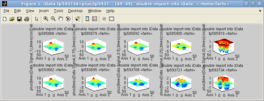
Linspace (first row) and logspace (2nd row)
The colon operator a:b is the same as linspace with a number of steps
which is the integer difference between the objects mean value.
Interpolation,
smoothing, intersection and union
Most binary operators require to interpolate the objects onto common
axes prior to applying the mathematical operation. The common axes
may be obtained from intersection or union of object axes.
The interpolation method used is based on a Delaunay
triangular multidimensional tessellation (using the Computational Geometry Algorithms
Library, CGAL).
Intersection and
union
The intersect and union binary operators determine
the minimum and maximum axes bounds, as well as a axes binning. The
inner and outer values are returned by
the intersect and union methods resp. Resulting objects are
interpolated, using the interp
operator, onto this new axis system, so that binary operators are
easy to apply afterwards.
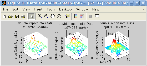
In the following example, we shift an object along axes, and signal
value, and then show the intersection and union. Extrapolated
values, for union, are set to 0.
>> a = iData(peaks);
>> b = copyobj(a);
>> a{1} = a{1}+10; a{2} = a{2}+10;  % shift along X and Y
>> a.Signal=a.Signal+5;             % shift along Z
>> [ai,bi]=intersect(a,b);
>> [au,bu]=union(a,b);
>> subplot(1,3,1); plot([a  b ],'transparent tight')
>> subplot(1,3,2); plot([ai bi],'transparent tight')
>> subplot(1,3,3); plot([au bu],'transparent tight')
Interpolation
The interp operator can be
used to interpolate one object onto an other axis coordinate frame,
which can be given as an other object, a binning scaling factor, or
a set of axes. The interpolation method can be specified as an
additional character argument amongst linear (default), cubic, spline, nearest.
>> a = iData(peaks(10))+2
>> b = interp(a,2)	% doubled binning, but we rather recommend the 'resize' method (see below)
>> c = interp(a,1:.25:15,3:.25:12)
>> subplot([a b c],[1 3],'mesh tight')

Event data
sets
It is possible to create an event data set from a column-type
object (that is a matrix which columns are axes/data) by means
of the '
event' method (which creates a cloud of points)
or the '
hist' method (which creates an histogram out of
an event list).
For event based data sets, the
hist
operator transforms the event object into an histogrammed data
set. The histogram axes can be given as vectors (where event
will be accumulated), or a number of bins within the [min max]
of the distributions. The
hist
operator is much faster than the interpolation one,
interp
for event based data.
>> a=iData([ ifitpath 'Data/Monitor_GV*']);
>> b=hist(a);
>> surf(b, 'median');
If the number of events is limited compared to the number of
bins in the histogram, some areas of the histogram can remain
empty when filling it with the events. It is then possible to '
fill'
the empty slots with a fast neighboring algorithm, using a
discrete cosine transform.
>> a=iData([ ifitpath 'Data/Monitor_GV*']);
>> b=hist(a);
>> c=fill(b);
>> subplot(a,b,c);
Re-binning
and resizing
To compress an object and reduce its binning, that is the number
of elements on each dimension, you can use the
reducevolume method. Without
argument, it reduces the number of elements to less than 1e6.
Additional arguments indicate the compression factor on each
dimension. This method is automatically used when plotting large
objects (except if the plot options contains a
'full' or
'whole' word).
In a similar manner, the
resize
method is a very fast yet accurate algorithm (
discrete
cosine transform) to make a fast rebinning, that is change
the number of elements on each dimension/rank, but preserve the
data set meaning.
>> a = iData(peaks(40))+2
>> subplot(a, resize(a, [20 20]), resize(a, 40, 40)) % resize operation
This allows for instance to quickly reduce the dimensionality of
a data set:
>> b = iData(flow);
>> resize(b, [25 50 1]);	% makes a 2D object from a 3D one
Reference:
Narasimha M. et al,
On
the computation of the discrete cosine transform, IEEE
Trans Comm, 26, 6, 1978, pp 934-936.
Smoothing
To explicitly smooth a data set, you can use the '
smooth' method, which makes
use of a discrete cosine transform filter spline smoothing
(shape preserving):
>> a = iData(peaks(40).*(1+0.1*randn(40)));
>> b = smooth(a);
>> subplot(a,b);
Reference:
Garcia D, Robust smoothing of gridded data in one and higher
dimensions with missing values.
Computational Statistics & Data Analysis,
2010.
The smoothing can also use a
Savitsky-Golay
moving average, but may lead to significant sharp features
modifications (be cautious).
>> b = smooth(a, 'sgolay');
>> b = smooth(a, span, 'sgolay', degree); % Savitsky Golay degree and span (length) specified
Last, you can use a
nD Gaussian
blur
>> b = smooth(a, 'gauss',1);		% Gaussian smoothing, all width=1
>> b = smooth(a, 'gauss',[ 1 10 ]);	% idem, with specific width, here for a 2D smoothing
Last, in the case a data set contains NaN (Not-a-Number) values
(that is missing values), you can fill these values with a fast
interpolation on neighboring elements using the
fill
method (based on a
discrete
cosine transform).
Manipulating
object dimensions
It is also possible to manipulate an object Signal in the same
way as a matrix with methods
reshape
(re-order elements in the object)
, permute (permute ranks, that is a generalized
transposition) and
circshift
(shift ranks/dimensions), which work just as their matrix
equivalent.
Last, the
sort operator
sorts object axes, in ascending or descending order. The
corresponding Signal, Error, and Monitor values are also
re-ordered accordingly.
E.
Farhi
- iFit/Math operators - Aug. 22, 2017
1.10 -
back to
Main iFit Page 
 The Fourier
Transform operators fft
and 'inverse' ifft perform
a Discrete FFT computation from an N-dimensional object. The axes
are converted to frequency/reciprocal axes.
 The gradient
operator computes the partial derivatives
∇ of an object. (see Gradient definition)
 The following
example adds a 2D data set with a 1D data set, which is extended.
The intersection selects only the positive axis values from the 1D
object, here in [0 5]. As the 2D object has no default Monitor (set
to 1), we set it to 1/10 of the corresponding mean value in the 1D
object (if not done so the IN6 data is under weighted compared with
the IN20 data for which Monitor is high). The magenta and blue
arrows indicate how the data is added, and the 1D data set extended
along the Axis 2. as shown
with the double arrow.
 When the 1st object has to be convoluted with
a response function (e.g.
instrument resolution function), the usual options to use should be:
 This
method works remarkably for signals with sharp peaks. The following
example displays the automatically found peaks on top of the object
view:
 There are a
number of methods used to extract projected and summed objects.
Technically, the projection on one axis is the sum along all other
axis.
  which will reduce the dimensionality, and be
roughly equivalent to sum
when dx=1.
 In the following example, the object d is the concatenation of 4
objects [a b c d],
sequentially. The concatenation of the 4 axes in 'd' is the repetition of the
initial axis. We then create an 'f'
object for which the axis is reset to the default, showing indeed
the concatenation of objects. Last, we assemble the same data set
side by side onto a new dimension, creating a surface 'g'.
 Similarly to the cat, the dog operator
splits an object into slices along a given dimension, returning an
array with as many elements as the length of this dimension. This is
the opposite to the cat
(of course !).