iFit: importing data into objects
- Importing data from a file (iData,
load)
- Distant files (http://, ...)
- Compressed files (.zip, ...)
- Anchor references (file#anchor)
- Setting Signal and Axes when
they are not set properly
- Supported data formats
- Example data files
- Importing directly from Matlab
variables
- Importing from Matlab Figures
- How it works (looktxt, iLoad,
Loaders)
Importing data from
a file (iData,
load)
This is done by converting a file path to an iData
object, or directly with the
iData/load method. The ifitpath points to the iFit
library location.
>> a = iData([ ifitpath 'Data/ILL_IN6.dat' ]);
>> a = load(iData, [ ifitpath 'Data/ILL_IN6.dat' ]);

>> a = iData + [ ifitpath 'Data/ILL_IN6.dat' ];
As seen in the last example, when performing a binary operation with
a file name (here an empty object added with a file name), the
corresponding file is imported.
These commands result in the following output, which produce an
iData object:
iLoad: Importing file iFit/Data/ILL_IN6.dat with method ILL Data (normal integers) (looktxt)
looktxt iFit/Data/ILL_IN6.dat --headers --fortran --catenate --fast --binary --makerows=IIII --makerows=FFFF --outfile=/tmp/lk_915264556_CZi4aN
Warning: Data root level renamed as lk_915264556_CZi4aN (started with number).
         Output file names are unchanged [looktxt:file_open:1377]
Warning: File 'iFit/Data/ILL_IN6.dat' c='-' [num pos=250] two fortran numbers are touching each other
Warning: File 'iFit/Data/ILL_IN6.dat' c='-' [num pos=2086] two fortran numbers are touching each other
Warning: File 'iFit/Data/ILL_IN6.dat' c='-' [num pos=2086] two fortran numbers are touching each other
Warning: File 'iFit/Data/ILL_IN6.dat' c='-' [num pos=2107] two fortran numbers are touching each other
Warning: File 'iFit/Data/ILL_IN6.dat' c='-' [num pos=2127] two fortran numbers are touching each other
Looktxt: file 'iFit/Data/ILL_IN6.dat': wrote 9 numerical fields into /tmp//lk_915264556_CZi4aN.m
iData: Setting the Signal of tp481575 to the biggest numerical field Data.IIIIIIIIIIIIIIIIIIIIIIIIIIIII_13 with length 131584.

a =  iData object:

    [Tag]     [Dimension]                           [Title] [Last command]          [Label]
 tp481575      [257  512] 'File ILL_IN6.dat ILL Data (n...' tp481575=load(iData,...
|
Wildcards (*,?) are supported. The file separator symbol ('/' for
Linux/Unix/MacOSX and '\' for Windows) is automatically adapted to
the system used.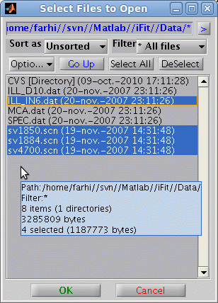
Directory may be imported (and thus all files therein) as well as
lists of files (given as a cell of strings {...})
>> a = iData( [ ifitpath 'Data' ]);
>> a = iData({ [ ifitpath 'Data/*.dat' ] ,...
[ ifitpath 'Data/sv1850.scn' ],...
[ ifitpath 'Data/sv1884.scn' ],...
[ ifitpath 'Data/sv4700.scn' ] });
which returns an array of iData objects.
A file selector, which
supports multiple file selection, may be used by issuing
>> a = iData('')
>> a = load(iData,'')
The choice of the file selector style can be done in the iLoad configuration (refer to
the Loaders page).
By default, an analysis of the file name extension and the file
content will be done, and the best importer method will be used. It
is possible to select a preferred method with e.g.
>> a = load(iData, 'filename', 'HDF5')
>> a = load(iData, 'filename', 'gui'); % a method selector pops-up.
A list of the supported formats is shown below.
The resulting objects will usually be 1D, 2D, 3D, nD histograms or
nD event lists. Refer to the iData and Math page to learn how to manipulate these
objects (set, get, setalias, getalias, setaxis, getaxis), and in
particular how to reduce/extend their dimensionality (sum,
indexing, ...), or convert events into histograms (hist,
interp).
Distant files
(http://, ...)
The specified file names may include URL tags such as
- file://filename
- ftp://filename
- http://filename
- https://filename
were the two latter cases first get a copy of the distant file
(requires local write permission), and then import it. A valid
Internet connection is then required, with proper Proxy settings if
needed.
Compressed files
(.zip, ...)
Compressed files (ZIP, TAR, GZIP, Z) can also be imported directly,
in which case they are first extracted locally (requires write
permission), and then imported. This extraction mechanism also
applied for distant file.
Anchor references
(file#anchor)
The file name may end with an anchor reference using the '#'
character, such as in
[ 'file#Data' ]
// import only parts which mention Data in
file
'http://path/file.zip#Data'
// import only Data in the extracted archive
In this case, the anchor is searched in the imported data, and only
the corresponding matching elements are returned. The resulting
objects are thus smaller in size.
In the case a directory is given, the anchor can be used to restrict
the recursive import of files, using a token to search in file
names, such as
[ directory 'ILL'
] // import only files which contain 'ILL'
in their names, with recursive search
If only one level exists in the directory, then this is equivalent
to importing 'directory/*ILL*'.
Setting Signal and
Axes when they are not set properly
There may be cases for which the reading of the file is done
properly, but the Signal, Error and Axes are set to their default
values, that is the largest numerical block as the Signal, the sqrt(Signal) as the Error, and
simple indices as Axes. In this case it may be appropriate to
customize the appearence of the scientific data set by setting the
Signal, Error aliases, and defining the Axes values.
In order to identify where the Signal and Axes may be stored in the
object, you should start by displaying the Data content of the
object:
>> a = iData([ ifitpath 'Data/ILL_IN6.dat' ]);
>> a.Data			% displays the whole object Data structure, as read from the file and stored in memory
ans =
    RRRRRRRRRRRRRRRRRRRRRRRRRRRRRRRR: [142198 0 1]
    AAAAAAAAAAAAAAAAAAAAAAAAAAAAAAAA: [2x1 double]
    IIIIIIIIIIIIIIIIIIIIIIIIIIIIIIII: [342x1 double]
    IIIIIIIIIIIIIIIIIIIIIIIIIIIIII_3: [1x156 double]
    FFFFFFFFFFFFFFFFFFFFFFFFFFFFFFFF: [2x1 double]
    FFFFFFFFFFFFFFFFFFFFFFFFFFFFFF_7: [1x384 double]
    FFFFFFFFFFFFFFFFFFFFFFFFFFFFF_10: [1x128 double]
    IIIIIIIIIIIIIIIIIIIIIIIIIIIII_13: [1x512 double]
    SSSSSSSSSSSSSSSSSSSSSSSSSSSSSSSS: [340x4 double]
    IIIIIIIIIIIIIIIIIIIIIIIIIIIII_17: [340x1024 double]
                          Attributes: [1x1 struct]
In this example, we have highligthed in red what we shall use as Signal and Axes.
Then, we just define:
>> a.Signal = 'Data.IIIIIIIIIIIIIIIIIIIIIIIIIIIII_17';
which sets the definition of the Signal
Alias as a link to the IIIIIIIIIIIIIIIIIIIIIIIIIIIII_17 field
in the Data member of the object, of size 340 rows by 1024 columns.
Letting the Error to its default empty definition assigns it to sqrt(this.Signal),
but you may define it as a link to a part of the Data, just as for
the Signal. The Signal
label can optionally be defined as
>> title(a, 'Signal label');
In order to define the Axes, they can be defined similarly as the
Signal:
>> a{1} = 'this.Data.SSSSSSSSSSSSSSSSSSSSSSSSSSSSSSSS(:,1)'; % defines the 1st axis as a link to the Data
where we make use of the this self reference in the link
(meaning find in myself), which allows expressions instead of simple
static links as for the Signal. This way we define the 1st axis as
the first column of the SSSSSSSSSSSSSSSSSSSSSSSSSSSSSSSS
field. It should have the proper dimension, in this example 340.
In this example, the second Axis of this 2d object has is not part
of the Data. We may then define it as a numerical value with e.g.
>> a{2} = linspace(0.001, 0.003, 1024);
which is a 1024 element vector from 1 to 3 ms. The Axis labels can
be set with e.g.:
>> label(a, 1, 'angle channel [1]')
>> label(a, 2, 'tof [ms]')
The final object is now fully described, and ready to be plotted,
fitted, and tortured...
Supported data
formats
In principle, any text based file is loaded transparently (see below). Binary files require a
dedicated wrapper, but many formats are supported. In some case,
additional axis definition specific to the format will be applied.
The list of available methods is usually stored in the iFit/Librarires/Loaders/iLoad_ini.m
file,
and can be obtained from the iLoad function
>> iLoad('formats'); % or: iData('formats')
A local iLoad.ini
configuration file may be stored in the Matlab Preferences directory, which
then overrides the system default (refer to the iLoad configuration help
page).
The current supported format list is (details in Loaders):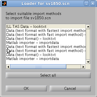
- any Data in text format
- ILL Data (legacy, text, most instruments at the ILL)
- ILL TAS Data (legacy, text, polarized or not)
- ILL Cyclops
neutron Laue diffractometer image (HBIN)
- Chalk River CNBC
NRU data, including multi-wire and polarized data
- SPEC ESRF
- McStas (Scan DAT output,
1D, 2D monitor, event lists, sim file, Sqw, LAZ, LAU tables)
- ISIS/SPE and SQW tof data (see Horace and LibISIS)
- INX tof data (ILL processed
TOF)
- ESRF data format (*.edf)
- Xray/neutron diffraction Crystallographic
binary file (*.cbf)
- MRI
3D volume Analyze 7.5 (*.hdr with associated *.img)
- NifTI medical imaging
volume data format (*.nii)
- NeXT/SUN (.au) sound
- Microsoft WAVE (.wav) sound
- Audio/Video Interleaved (*.avi)
- NetCDF
(*.nc)
- CDF (*.cdf)
- FITS (*.fits) used in
astronomy
- Microsoft Excel (*.xls)
- Image/Picture (*.gif, *.bmp, *.tif, *.jpg, *.png, ppm, pgm,
pbm)
- HDF4 (*.hdf4)
- HDF5 (*.hdf5) including
the NeXus format (*.nx,
*.n4, *.ns, *.n5, *.nxs) and more specifically Mantid workspaces.
- Matlab workspace (*.mat) a customized HDF
- Comma Separated Values (*.csv)
- Numerical single block (*.dlm)
- XML (*.xml)
- FIG (Matlab figure, *.fig)
- Protein Data Bank (*.pdb)
- STL
stereolithography (*.stl)
- OFF
object geometry (*.off)
- PLY
Polygon File Format or the Stanford Triangle Format (*.ply)
- MAR MarResearch CCD
Camera (*.mar, *.mccd), a variant of the TIFF format
- SIF
Andor SIF CCD Camera (*.sif)
- SPE
Princeton/Roper Scientific WinView CCD / PI Acton Camera file
(*.spe)
- IMG ADSC
Quantum CCD Camera (*.img)
- CIF,
CFL/PCR, INS/RES/SHX
Crystallography files (FullProf, ShelX)
- EZD, MRC and CCP4
electron density maps (*.map, *.ezd, *.ccp4)
- YAML and JSON (*.yaml,
*.yml, *.json)
- NMR Bruker, Varian and JEOL data files
- IBW Igor Wave data
file (*.ibw)
- OBJ
Wavefront 3D (*.obj)
- LabView LVM
and TDMS
files (*.lvm; *.tdms)
- Bruker FT-IR OPUS
data files (*.0001, *.0002, ...)
- LLB TAS binary data files (R* and C*)
- IDL
SAV data (*.sav)
- DAT Quantum
Design VMS ppms/mpms
- XVG XmGrace
data set
- Agilent Mass Spectrometry (*.CH, *.D, *.MS)
- Thermo Finnigan Mass Spectrometry (*.RAW)
- ENDF
Evaluated
Nuclear Data File (*.endf,*.tsl)
- ACE MCNP files (*.ace)
[requires PyNE]
- Numpy NPY
binary array (*.npy)
- VASP POSCAR
file for molecular modelling
- HP/Agilent/Keysight Standard Data Format (*.SDF)
- SPINWAVE
(LLB) input file for sqw_spinwave
- Sqw 4D data set for McStas Single_crystal_inelastic component
(*.Sqw4)
A detailed list of format descriptions can be found in the Loaders help
pages, as well as the procedure
to be used to define new data formats. Some of these formats are
also available for Saving iData objects.
To force a file to be imported with a specific data format, specify
the format description or extension as listed from the iData('formats')
output e.g.:
>> iData('formats')
...
PDB        read_pdb/load_xyen  Protein Data Bank
...
>> iData('filename','Protein Data Bank')
>> iData('filename','PDB')
If you can not import a reluctant text
file, try the most tolerant text reader configurations:
>> iData('filename','text format with fast import method')
>> iData('filename','Data (text format)')
will import the raw content, without post formatting of the object
in memory. You will probably need to assign manually some of the
Signal and Axes (see iData object help).
If you want to tune the way a text file is read, read the 'Unsupported data formats'
section in the Loaders page. You can for instance handle wrapped
lines, specific tokens to search for, automatic append mode, ...
A typical, usage would be:
>> a=iData(filename, 'text','--catenate','--fast','--headers','--wrapped', ... other options);
The full list of options for text files can be obtained with:
>> iLoad(' ','text','--help')
It may also be that the looktxt
MeX file is corrupted. Refer to the Changes/Bugs and Install pages.
Example data files
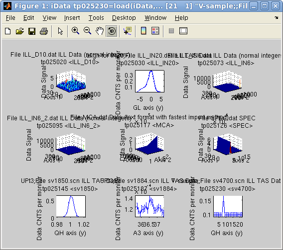 The iFit package provides a set of example data files used to demonstrate the
functionality of the package. The description of each format is in Loaders.
- ILL_D10.dat:
some D10 neutron
diffractometer measurement at the ILL [text]
- ILL_IN20.dat: some IN20 neutron triple-axis
diffractometer at the ILL (GL goniometer scan) [text]
- ILL_IN6.dat:
some IN6 neutron time of
flight spectrometer at the ILL (liquid water) [text]
- ILL_IN6_2.dat: some IN6 neutron time of flight
spectrometer at the ILL (liquid 3He) [text]
- MCA.dat:
some Canberra multichannel analyzer data (from a Sandercock
Brillouin light scattering spectrometer) [text]
- SPEC.dat:
some ESRF data, old SPEC format [text]
- sv1850.scn:
some IN12 neutron
triple-axis diffractometer at the ILL (QH scan) [text]
- sv1884.scn:
some IN12 neutron
triple-axis diffractometer at the ILL (sample rotation scan)
[text]
- sv4700.scn:
some IN12 neutron
triple-axis diffractometer at the ILL [text]
- Example.spe:
an ISIS SPE file from a TOF spectrometer (from the Mantid Project) [SPE]
- 30dor.fits:
30Dor Spitzer IRAC 8um image from SAGE [binary, FITS format]
- Ag_3_a.edf:
an image of an algae cell [binary, ESRF EDF format]
- Ag_3_a.hdf4:
an image of an algae cell [binary, HDF4 image]
- peaks.hdf5:
a surface stored as an HDF5 file [binary, HDF5]
- SQW_coh_lGe.nc: the coherent dynamic
structure factor obtained from
ab-initio molecular dynamics (VASP) and
analyzed with nMoldyn
[binary, NetCDF]
- IRS21360_graphite002_ipg.nxs:
an ISIS/IRIS
high resolution TOF spectrometer (NeXus file from the Mantid Project)
[binary, HDF5/NeXus with compression]
- peg268.csv:
an example Comma Separated values files from Excel [text].
- YIG_4A_corr_vana_spectre.inx:
an INX example file obtained from IN5 tof at the ILL [text,
INX].
- cyno_atlas.4dint.hdr
and cyno_atlas.4dint.img:
Tomographic monkey brain data - Volume dataset in Analyze
format. Open the 'hdr' file.
See ReadAnalyze
[binary]
- insulin_pilatus6mconverted_orig.cbf:
a CBF insulin small angle scattering pattern, e.g. from cSAXS@SLS
[binary, CBF]
- rita22010n021140.hdf:
a RITA2@PSI
data file [binary, HDF5/NeXus with compression]
- PDBSilk.pdb:
an example PDB file [text, PDB]
- nano_50K_4.8a_03_h4.hdf:
an inelastic scattering example from IN5 tof at the ILL [binary,
HDF4/NeXus with compression]
- Diff_BananaTheta_1314088587.th
and Diff_BananaPSD_1314088587.th_y:
example McStas simulation
result files, 1D and 2D [text, McStas]
- Monitor_GV_1330447143_list.L.x.y.z:
a list of events simulated with McStas, for the L3
strain-scanner at CNBC
NRU [text, McStas]
- AL20_017.DAT:
example data files from the D3 reflectometer at Chalk River CNBC NRU [text]
- nac_1645179.dat:
a D20@ILL diffractogram of a Na2Ca3Al2F14 powder [text]
- Na2Ca3Al2F14.cfl:
a NaCaAlF standard powder used to calibrate neutron
diffractometers [text]
- 111107AgBH.0001.mccd:
an X-ray MarCCD image [binary/TIFF]
- Q1_Test_Protein.img: an
X-ray ADSC CCD Camera [binary]
- gluco_toluene.0001:
an OPUS file [binary]
- simple_test.tdms:
a LabView TDMS file [binary]
- C004 and R014: LLB TAS [binary]
- POSCAR_MgO: a VASP
system configuration for MgO insulator [POSCAR]
- POSCAR_SrTiO3: a
VASP system configuration for SrTiO3 insulator [POSCAR]
- POSCAR_NaCl: a VASP
system configuration for NaCl insulator [POSCAR]
- POSCAR_AlN: a VASP
system configuration for AlN insulator [POSCAR]
- POSCAR_Al: a VASP
system configuration for Al metal [POSCAR]
- 008545.spe: an ISIS
SPE file from a TOF spectrometer (from IN5@ILL) [SPE]
- LaMnO3 and MnFe4Si3 spinwave
input file for sqw_spinwave [text]
All of these can be directly accessed with e.g.
>> b = iData([ ifitpath 'Data/' filename ]);
>> a = iData([ ifitpath 'Data' ]);
>> subplot(a, 'tight')
The empty iData object ∅ can be obtained from:
>> a=iData
>> a=zeros(iData, size)
Importing directly
from Matlab variables
A direct import of a Matlab variable is performed with
>> a = iData(variable)
such as
>> a = iData(rand(10))
or
>> a = iData(struct('a',1,'b','a string'))
This works for basically any input object (structure, numeric array,
cell, ...).
In addition, it is possible to evaluate an iFunc
model, and create an iData of it:
>> g = gauss(5); 		% an iFunc Gaussian with initial width=5
>> a = iData(g, [], -5:5);	% evaluate the model with its current parameters
A special syntax is available to import Signal and Axis definitions
with e.g.
>> a = iData(x,y,...c);
imports Signal as 'c' and
axes x,y, ...
The Error, defaulted to sqrt(Signal),
may be defined as well using e.g.:
>> a.Error = 'Data.myErrors'; % define the Error alias as a link inside the Data
where myErrors should be
found in the object Data. Identify it by displaying it with e.g.:
>> a.Data
Refer to the Setting Signal and
Axes when they are not set properly help in order to customize
the appearence of the object.
The findobj
method can be used to inquire for all iData objects available in the
workspace/memory:
>> a = findobj(iData);
The zeros method
initializes an empty (or constant) array of objects:
>> a=zeros(iData, size)  % create a [size] array of empty objects
>> a=zeros(object, size) % duplicates 'object' as a [size] array
Importing from
Matlab Figures
The direct import method also works from Matlab figures, when simply
giving a valid Handle Graphics Object to iData:
>> f=figure; peaks;
>> a = iData(f);
The handle can be a figure, a surface, an axis, a line, ...
How it works
(looktxt, iLoad, Loaders)
The file names to import are sent to the Loaders/iLoad
routine,
which
scans
the
file
and
searches
for
the
file
extension
and
patterns
in
the
file
contents
(in
the
case
of
text
files)
in
order
to
identify
the proper importation method to use.
The text files are processed with the looktxt parser (refer to http://looktxt.sourceforge.net)
and translated into a Matlab script which is then read into the
workspace. Binary files are read with dedicated read routines, as it
is usually not possible to interpret correctly the file structure ab-initio.
The resulting Matlab variable is a structure, which holds a Data field with all numerical
blocks from the initial file, and a Header field which holds any preceding comment
strings for each field. Data fields are automatically named from
keywords/comments found just before the numerical blocks (in text
files).
The structures are then converted into iData
objects, and optionally some data format specific post-processing
scripts are applied, as described in Loaders/iLoad_ini.m.
When no Signal is defined, it is assigned to the largest numerical
block found in the file. The default axes are set as matrix indexes.
Refer to the Loaders documentation to
learn how to customize load methods and import filters.
E.
Farhi
- iFit/iData loading data - Nov. 27, 2018 2.0.2 - back to
Main iFit Page


 The iFit package provides a set of example data files used to demonstrate the
functionality of the package. The description of each format is in Loaders.
