In this document, we demonstrate how iFunc, iFit/Optimizers and iData objects can all be used transparently to simulate and optimize McStas/McXtrace neutron and X-ray ray-tracing Monte-Carlo instrument models.

To import a McStas simulation results, just use

>> results = iData('single_detector_file')
>> results = iData('directory')                 % import everything in the directory, including sim files (files may imported more than once)
>> results = iData('scan_directory/mcstas.dat') % for scans
>> results = iData('scan_directory/mcstas.sim') % for all files from the directory, uniquely.

which returns a single or an array of iData object(s), that you can plot with e.g. subplot.
The resulting McStas data has an additional Parameters field which holds the instrument parameters used for the simulation.

>> results(1).Parameters

Building an instrument model

The syntax for building a McCode (McStas for neutrons or McXtrace for X-rays) instrument model is:

>> model = mccode('instrument');	% uses the given instrument file (*.instr)
>> model = mccode('gui');		% lists all available instruments to select one
>> model = mccode('');			% pop-up a file selector to select an *.instr file
>> model = mccode('defaults');		% uses the templateDIFF instrument as example 

which compile the instrument, and create an iFunc model (in fact an iFunc_McCode flavour).
When the instrument is not found in the current directory, it is searched in the McStas/McXtrace library (may be specified with the MCSTAS and MCXTRACE environment variables), and eventually copied locally, which triggers its compilation.

In addition, it is possible to select an instrument from the McStas/McXtrace installation with:

model = mccode('gui')

You may even assemble these models as iFunc arrays to iteratively perform series of simulations, or use arithmetic operations to combine models (see the iFunc documentation).

The resulting 'model' object can be forced into an iFunc_McCode one (in case its flavour was lost) with:

• model = iFunc_McCode(model)

This type of sub-class (derived from iFunc), provides all iFunc methods, but also specific methods adapted to McCode simulations:

• plot(model)

plot the model geometry in 3D.

• feval(model)

evaluate the model using its current parameter values and settings. The returned data is an array for the selected or last Monitor value. Other monitors are available as iData objects in model.UserData.monitors

• edit(model)

edit the instrument source code. Do not forget to save the file before closing the editor. If changes are done, the object is updated, and the instrument is re-compiled.

• dialog(model)

displays a table where you can change the parameter/configuration values. Instrument parameters (scalars) can be given as a single scalar, or a vector (for scans). The calculation starts when you close the table. To Cancel the computation, select the contextual menu (right mouse button) CANCEL item, or press Ctrl-C at the prompt. The resulting monitors are displayed when the simulation end.

• publish(model)

create a full readable report as an HTML web page, including the instrument model view, results, and code.

It is also possible to finely tune the instrument configuration using standard McStas/McXtrace options with the syntax:

>>  mccode('instrument', options)

and the following options:

options.dir	directory where to store results, or set automatically (string) ; the last simulation files are stored therein 'sim'.
options.ncount	number of neutron events per iteration, e.g. 1e6 (double).
options.mpi	number of processors/cores to use with MPI on localhost or cluster (integer) ; when MPI is available, and mpi options is not given, all cores are then used. Use options.mpi=1 for a serial calculation.
options.machines	file name containing the list of machines/nodes to use (string), as often found in cluster job schedulers.
options.seed	random number seed to use for each iteration (double)
options.gravitation	0 or 1 to set gravitation handling in neutron propagation (boolean)
options.monitor	a single monitor name pattern to read, or left empty for the last (string). The whole monitors are available as iData objects in the model.UserData.monitors field. Wildcard expression can be used. See below for more advanced customisation.
options.mpirun	set the executable path to 'mpirun', or automatically found when not set. Set it to 'none' or set options.mpi=1 to not compile with MPI.
options.compile	0 or 1 to force re-compilation of the executable.

 
The options can be given as a structure or as a string, e.g. 'ncount=1e6; compile=1'.

NOTE: if the instrument can not be built, force the compilation with:

>>  mccode('instrument', 'compile=1')

as a previous executable may be in the way, and block the generation of the new model.

The scalar instrument parameters of type 'double' are used as model parameters.
Other parameters (e.g. of type string and int) are stored as a structure in:

• model.UserData.Parameters_Constant

The options ncount, seed, gravitation, monitor can be changed after the model creation in the UserData area of the object e.g.:

• model.UserData.options.gravitation=1;
• model.UserData.options.monitor='*Theta*';

Specifying which monitor to use

The default behaviour is to leave options.monitor left unset at the model creation, so that all monitors are read when simulating instruments. The last monitor is then used as model value. This provides maximum information, but the processing overhead time is increased due to more data handling compared to a single/restricted monitor name selection.

• model=mccode('templateDIFF');  % same as mccode('defaults')

In order to improve the computational efficiency, it is advised to specify which files have to be imported to define the model value by giving a file name or pattern (wildcard patterns can be used). This specification can be done either when building the model:

• model=mccode('templateDIFF','monitor=Diff_BananaPSD*');

or afterwards:

• model=mccode('templateDIFF');
• model.UserData.options.monitor='*BananaPSD*'

which in both cases will select monitor files which match the given string as an exact file name or match the pattern when using a wildcard expression ( '*Theta*' ). In case the selection brings multiple files, the last one is used. When the monitor name selection does not match any file, or is given as empty, all monitors are imported, and the last one in the list is used.

All selected monitors are imported as iData object(s), in:

• model.UserData.monitors

In practice, you will often either not specify the 'monitor' at the model creation to leave the system select the last one, or indicate a specific monitor name/pattern of your choice.

Customize the model value
In addition, you may customize how to use the monitor data either by adding expression after the initial filename/pattern, or by extending the model after its creation.

The monitor to use as optimization criteria (options.monitor) can be part of a more complex expression, which still must start with the file name/pattern to select the monitor(s) and then refer to itself with the 'signal' variable (which are iData object(s)), such as in the following example where we sum all selected monitors from the pattern (when more than one are found), and define the criteria as Amplitude/width² (for a single peak):

>> options.monitor='*Banana_Theta*; signal=plus(signal); signal=max(signal)/std(signal)^2;'
>> model=mccode('templateDIFF', options)

The options.monitor can be given in a compact way if the file pattern and the expression are enclosed in single or double quotes, such as in:

• model=mccode('templateDIFF','monitor="*Theta* signal=max(signal)/std(signal)^2"');

An other possibility (less recommended) is to extend the model after its creation:

• model = mccode('templateDIFF','monitor=Diff_BananaPSD*');
• model = model + 'signal=max(signal)/std(signal)^2';
  

Requirements

As iFit contains powerful import routines, that support McStas/McXtrace data files, it is straight forward to launch a McStas/McXtrace instrument simulation from Matlab and get back the simulation results. To do so, you will obviously need to have iFit installed (refer to the Install page), as well as McStas (refer to the McStas web site) or McXtrace. When used with the standalone version, no Matlab license is needed. To use all the CPU cores, you need to have installed an MPI library, e.g. OpenMPI.

Running a single simulation

The model value is corresponds with the 'options.monitor' selected, i.e. the last one, or a specific name pattern. This selection can be changed any time without rebuilding the model (see above).

The instrument can be evaluated with given parameters and optionally axes:

>> results = feval(model);			% return the monitor, using current/default parameters
>> results = feval(model, parameters);		% return the monitor as an array using guessed axes
>> results = feval(model, parameters, x,y,...);	% return the monitor as an array, using specified axes
>> results = feval(model, parameters, nan);	% return the raw monitor as an array

but it may be more convenient to manipulate the model value as iData objects:

>> result = iData(model, parameters);		% return monitor interpolated onto guessed axes
>> result = iData(model, parameters, nan);	% return raw monitor as an iData object
>> result = iData(model, parameters, x,y,...);	% return monitor interpolated onto axes x,y,...
>> plot(result);
>> plot(model.UserData.monitors)

where parameters is a structure, or string, or vector that holds parameter names and values, e.g.

Running series of simulations (scans)

You may scan the model parameters when they are assigned as vector.

• model=mccode('templateDIFF');
• parameters.RV = 0.5:.05:1.5;
• scan = iData(model, parameters);

A more compact way can be used, using explicit scan values and axes:

• model=mccode('templateDIFF');
• scan = iData(model, 'RV=[0.5 1 1.5]', -.15:.05:.15, -5:50);

The argument returned is an iData object array containing the model monitor as a function of the scanned parameters. You may compute the integral value with the 'sum' method:

>> integral = sum(scan, 0);

which can be directly plotted with e.g. 

>> plot(integral);     % simple plot, or median surface for multidimensional scans
>> scatter3(integral); % coloured points (possibly in 2D,3D)
>> plot3(integral);    % coloured lines in 2D, or volume for multidimensional scans
>> slice(integral);    % only for 3D scans, use slice-o-matic for volume inspection

You may as well concatenate the scan steps into a higher dimensionality volume using e.g. the iData/cat method:

>> catenated = cat(scan, 2);

Multidimensional scans are also possible. In the following example, we launch a quick 2D scan with parameters specified as a structure:

>> model = mccode('templateDIFF','monitor=Diff_BananaTheta');
>> scan = iData(model, struct('RV',[0.7 0.9 1.2],'L2',[1 1.3 1.5]), nan);

Then we may plot, as a 2D surface, the integral value for the model value monitor:

>> plot(iData(sum(scan,0)));

You may look at the instrument parameters used for the scans, e.g.

>> get(scan,'Parameters.RV')

Warning: Beware of the number of iterations required to scan large dimensionality spaces. In practice you should avoid spaces above 2 or 3 scanned parameters. Exceeding this will undoubtedly require very long computation times, and large memory storage.

You may also scan the non numerical parameters with e.g. for the 'powder' string parameter:

• scan=[];
• for vector = {'Na2Ca3Al2F14.laz','Al.laz','Ge.laz'}; model.UserData.Parameters_Constant.powder = vector{1}; scan = [ scan iData(model, [], nan) ]; end
• subplot(scan)

Running series of simulations (single step and scans): graphical user interface

A user interface can be used to enter most McStas/McXtrace configuration and instrument parameters. To display it, use:

• dialog(model)

which shows a table where instrument parameters can be specified as scalars (e.g. 1), vectors (e.g. [1 2 3] or 0:0.5:5 or linspace(0,5,10) ) or strings ('Al.laz' for the additional non variable parameters such as file names, etc).

Optimizing instrument parameters

The optimization of instrument parameters is performed as simply as a single simulation, using the fmax method to maximize the monitor value (you may similarly use fmin to minimize the model value).

>> best_parameters = fmax(model);		% maximize with the current/default parameters
>> best_parameters = fmax(model, parameters);	% maximize with given initial parameters

The parameters, as a vector, string or named structure, are initiated to their starting value, from which the optimization proceeds. An empty value requests to use the current/default values. Only numerical parameters can be optimized. Also, it is highly encouraged to use bounded parameters (that is define constraints, see below), else the optimizer can get lost, produce un-meaningful results, or return NaN parameter values.

You can tune the optimizer configuration, as explained in the iFunc documentation, with syntax:

>> best_parameters = fmax(model, parameters, options);

as well as any other optimizer configuration fields such as

• options.TolFun ='1%';      % stop when criteria changes are smaller that 1%
  
• options.TolX ='0.1%';       % stop when parameter changes are smaller that 0.1%
• options.Display='final';
• options.OutputFcn='fminplot'; % plots the criteria and parameters evolution during the optimization. 
• options.optimizer='fminpso'
• options.MaxFunEvals=100

>> best_parameters = fmax(model, parameters, options, x, y, ...);

>> best_parameters = fmax(model, parameters, options, nan);	% use raw monitors

>> model = mccode('templateDIFF','monitor=*Theta*');	% monitor contains 'Theta'
>> fix(model, 'all'); 				% fix all but RV L2
>> model.RV='free'; model.RV=[0.5 0.8 1.5];	% set RV bounds and value in a single assignment
>> model.L2='free'; model.L2=[1 3 4];
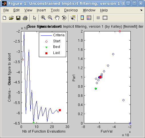
>> [parameters, fval, status, output]=fmax(model,[], 'optimizer=fminimfil; OutputFcn=fminplot', nan);

>> model = mccode('templateDIFF','monitor=*Theta*');	% monitor contains 'Theta'
>> fix(model, 'all'); 				% fix all
>> model.RV='free'; model.RV=[0.5 1 1.5];	% set RV free, bounds and value in a single assignment
>> [parameters, fval, status, output]=fmax(model,[], ...
  'optimizer=fminpso; OutputFcn=fminplot;TolFun =5%;TolX=5%;ncount=1e5;MaxFunEvals=100', nan);

	ans=
           0.8621