miFit: a user interface for iFit
- Starting
- Using specific miFit flavor
- Loading data and models
- from files
- from the Matlab/iFit prompt:
Data sets
- from the Matlab/iFit prompt:
Models
- from copy/paste
- from drag-and-drop
- from the TextEdit (File:Evaluate
code/script menu item)
- creating a new Data set
- creating new Models
- Working with Data sets
- Plotting data
- Sorting and searching data
- Selecting/deselecting regions of
interest (ROI)
- Mathematical operators on Data
sets
- Working with Models (fitting)
- Assigning and Evaluating Models
to Data sets
- Selecting a fit routine
(optimization algorithm)
- Fitting Models to Data sets
- Preferences
- Resetting miFit (default
Preferences)
- Saving your work
- Saving all data sets, Models
and Preferences
- Exporting selected Data sets
- Exporting Models (and importing
them as well
- Examples / Tutorials
- Fitting a simple peak
- Fitting a 'phonon' dispersion
(neutron_TAS)
This is the miFit help, a simple graphical user interface to
iFit. To access the main iFit help pages, click
here.
Starting
To start the miFit interface, just type 'mifit'
from the Matlab prompt when iFit is installed, or from the iFit
stand-alone prompt. The main window will then appear, as follows:
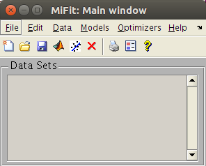 The miFit main window
The main window has menus, a toolbar with icons, and tips that show
up when bringing the mouse pointer over items. The imported data
sets are stored in a 'Data Sets' list.
On the first start-up, miFit builds a list of available
Models and Optimizers. This list can be re-built (updated) if you
reset the application from the Reset item in the File menu.
Before you reset miFit, it may be desirable to save your Data Sets.
Using specific
miFit flavor
miFit can be customized to provide specific features, from the Configurations
item in the File menu. Each configuration is an ini file
stored in the iFit/Applications/miFit/configurations
directory. You may add your own configurations there, based on the
existing ones. Selected configurations are appended to the current
Preferences, and saved for later use. They mostly populate new menu
items. In order to remove specific configurations from miFit, you
should Reset miFit as indicated below.
- neutrons_TAS: adds a Neutron Scattering menu
with 4D TAS resolution calculation and convolution. See below for an example usage.
- neutrons_Phonons: adds a Neutron
Scattering menu with 4D S(q,w) phonon capabilities (using e.g.
DFT codes). See here for more
details.
- neutrons_McStas: adds a Neutron
Scattering menu with instrument simulation using McStas. See here for more details.
Loading data and models
The imported Data Sets appear in the main miFit list.
The imported Models are inserted in the Models menu,
sorted by dimensionality (1D, 2D, 3D, 4D, others).
from files
The legacy way to import data files into miFit is to select the Open
item in the File menu. A file selector will pop-up, and
allow to select one or more data files (use Ctrl-click to select
files one-by-one, and Shift-click to select a range). You can
equally select the Open icon in the toolbar.
It is possible to import data files in any supported format
(whole list available in the Loaders
page). Once loaded, the data sets appear in the Data Sets list in
the main window.
Supported formats for Data Sets (stored as iData
objects):
- any Data in text format
- ILL Data (legacy, text, most instruments at the ILL)
- ILL TAS Data (legacy, text, polarized or not)
- ILL Cyclops neutron
Laue diffractometer image (HBIN)
- Chalk River CNBC NRU data,
including multi-wire and polarized data
- SPEC ESRF
- McStas (Scan DAT
output, 1D, 2D monitor, event lists, sim file, Sqw,
LAZ, LAU tables)
- ISIS/SPE and SQW tof data (see Horace and LibISIS)
- INX tof data (ILL processed
TOF)
- ESRF data format (*.edf)
- Xray/neutron diffraction Crystallographic
binary file (*.cbf)
- MRI
3D volume Analyze
7.5 (*.hdr with associated *.img)
- NifTI medical
imaging volume data format (*.nii)
- NeXT/SUN (.au) sound
- Microsoft WAVE (.wav) sound
- Audio/Video Interleaved (*.avi)
- NetCDF (*.nc)
- CDF (*.cdf)
- FITS (*.fits)
used in astronomy
- Microsoft Excel (*.xls)
- Image/Picture (*.gif, *.bmp, *.tif, *.jpg,
*.png, ppm, pgm, pbm)
- HDF4 (*.hdf4)
- HDF5 (*.hdf5)
including the NeXus format
(*.nx, *.n4, *.ns, *.n5, *.nxs) and more specifically Mantid workspaces.
- Matlab workspace (*.mat) a customized HDF
- Comma Separated Values (*.csv)
- Numerical single block (*.dlm)
- XML (*.xml)
- FIG (Matlab figure, *.fig)
|
- Protein Data
Bank (*.pdb)
- STL stereolithography
(*.stl)
- OFF object
geometry (*.off)
- PLY Polygon
File Format or the Stanford Triangle Format (*.ply)
- MAR MarResearch
CCD Camera (*.mar, *.mccd), a variant of the TIFF
format
- SIF Andor SIF
CCD Camera (*.sif)
- SPE Princeton/Roper
Scientific WinView CCD / PI Acton Camera file (*.spe)
- IMG ADSC
Quantum CCD Camera (*.img)
- CIF, CFL/PCR, INS/RES/SHX Crystallography
files (FullProf, ShelX)
- EZD, MRC and CCP4 electron
density maps (*.map, *.ezd, *.ccp4)
- YAML and JSON (*.yaml,
*.yml, *.json)
- NMR Bruker, Varian and JEOL data files
- IBW Igor Wave
data file (*.ibw)
- OBJ Wavefront
3D (*.obj)
- LabView LVM and TDMS files
(*.lvm; *.tdms)
- Bruker FT-IR OPUS data
files (*.0001, *.0002, ...)
- LLB TAS binary data files (R* and C*)
- IDL SAV data
(*.sav)
- DAT Quantum
Design VMS
ppms/mpms
- XVG XmGrace data set
- Agilent Mass Spectrometry (*.CH, *.D, *.MS)
- Thermo Finnigan Mass Spectrometry (*.RAW)
- ENDF Evaluated
Nuclear Data File (*.endf,*.tsl)
- ACE MCNP files
(*.ace) [requires PyNE]
- Numpy NPY
binary array (*.npy)
|
You can either import Models from the File:Open menu
item, e.g. as Matlab MAT workspaces containing iFunc objects, or using the dedicated Models:Import
menu item.
Supported formats for Models (stored as iFunc
objects):
- M Matlab script/function (*.m)
- MAT Matlab binary file (*.mat)
- JSON JavaScript Object Notation (*.json)
- YAML interchange format (*.yaml)
- XML file (*.xml)
from the Matlab/iFit prompt: Data sets
It is possible to work from the Matlab/iFit prompt, and send any numerical array, as well as iData (data sets) and iFunc (models) objects. This is done with the mifit(data) command. Any syntax from the Load page can be used, where 'mifit' stand in place of 'iData'.
To import a file, send it path: mifit(filename)
Remember to properly set the proxy settings in the Preferences in case you are behind one.
To import a numerical array: mifit(array)
a=rand(10);
mifit(a);
or mifit(x,y,z, ... signal)
x = 0:.1:8*pi; y = sin(x);
mifit(x,y);
or
a=[ 0 0
0.1000 0.0998
0.2000 0.1987
0.3000 0.2955
0.4000 0.3894
0.5000 0.4794
0.6000 0.5646
0.7000 0.6442
0.8000 0.7174
0.9000 0.7833
1.0000 0.8415
1.1000 0.8912
1.2000 0.9320 ];
mifit(a);
To import an iData object (data set. Refer to the Load page): mifit(iData)
a = iData(peaks);a.Title = 'Peak function'; label(a,1,'my X axis'); label(a,2,'my Y axis');mifit(a);
from the Matlab/iFit prompt: Models
To import a Model (iFunc object): mifit(iFunc)
f=gauss+lorz; f.Background_2=0; fix(f,'Background_2');mifit(f);
The new model is added to the 1D Models menu, as a blue entry, which is used to label 'user' models. Such models are 'static' in the sense that once in the Models menu, only the model parameters can be changed. These models are assigned a unique iD in the form iFxxxx.
It is also possible to add Models as expressions, which are then evaluated to create a model. Such models, shown in green in the Models menu, are 'dynamic' in the sense that they are used to effectively create other static models. Such model creators do not have a unique model iD. For instance, the 'sqw_phonons' model is dynamic. When called, it requires to enter parameters to initiate the model creation, such as the DFT code to use, the k-mesh, ... Then, a static model is created, but the parameters used initially (DFT, k-mesh, ...) can not be changed further. However, the model parameters (intensity, ...) can be changed, e.g. during fit processes.
To import a Model expression as a dynamic model (creator), use:
mifit('Models_Add_Entry','gauss+lorz');
from copy/paste
It is possible to use the Copy/Paste mechanism to import data sets. If the copied element is a file, it will be imported the same way as with the Open item above when selecting the Paste item in the Edit menu. You can also click on the grey window background or the 'Data Sets' label above the list, and press Ctrl-V (command-V on MacOSX)
You can also copy whole data blocks (e.g. numerical values/array from a text editor or a spreadsheet), and paste them into miFit.
The copy/paste also works with path name (as strings) including distant files (URL with http, https, ftp). Remember to properly set the proxy settings in the Preferences in case you are behind one.
from drag-and-drop
A very convenient way to import data is to drag a data file, and drop it into the miFit window. A new data sets object is then read, and added to the list. This works with multiple file selections, as well as file path given as strings, including HTTP, HTTPS and FTP links. Remember to properly set the proxy settings in the Preferences in case you are behind one.
from the TextEdit (File:Evaluate code/script menu item)
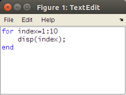 The miFit File menu has an Evaluate code/script menu item. Your can enter any Matlab command there, and evaluate a selection, or all ('Play' button or the TextEdit:File:Evaluate selection item) . To send some data directly to miFit, use e.g.:
just as you would do from the prompt.
creating a new Data set
You may create a new data set using a spreadsheet by selecting the New item in the File menu, or the white page icon in the toolbar. Type in your data (Copy/Paste works). The data set will be imported into miFit when you close the window.
creating new Models
The way to define new Models into miFit is via the Matlab/iFit prompt (see above), or by importing a data file containing a model (iFunc) definition.
Working with Data sets
You should first import or create Data Sets (see above), which populate the miFit list. Each entry is an iData object.
Most actions require to select one or more Data Sets from the list. You can use the mouse click, with the Ctrl key for adding one-by-one, or the Shit key to add in a range. The Select All item in the Edit menu allows to select all, or none (when they are all selected). To deselect a single item, use mouse Ctrl-click on it. You can use Ctrl-A to select all.
Subsequent Data Sets states are saved into a History, which allow to Undo last operations (data states, model selections, etc...). You may as well save any time the miFit state from the Save as item in the File menu.
The miFit interface provides, in its miFit:File:Evaluate code/script menu item, access to the TextEdit application, which allows to write scripts and commands, and execute them (TextEdit:File:Evaluate).
This is highly recommended when using the standalone iFit executable, as you can keep track of all your commands as a
script, with highlight syntaxing, and it is not sensitive to the
localised character crash [bug 624817].
Plotting data
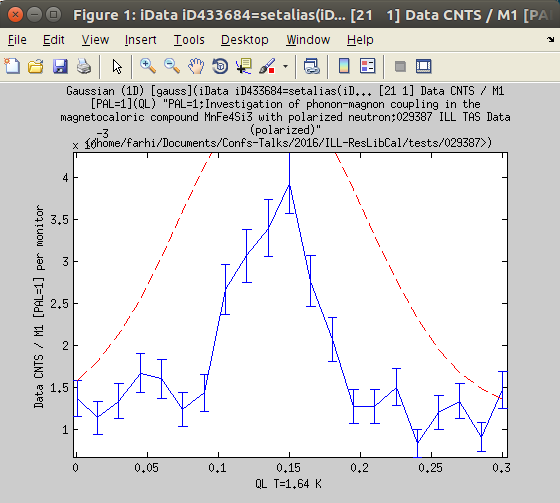 You can plot Data Sets by selecting one or more, and then click on the Plot icon in the toolbar, or the Plot item in the Data menu. To plot a single Data Set, double-click it in the Data Set list. Data Sets with assigned Models (see below) will also show the model evaluation.
You can of course export the plot windows from their File:Save as menu item, and print them subsequently.
To print a data set, we recommend to use the printer icon in the tool bar, or the File:Print menu item on a selection of Data Sets. A web page will be generated, displayed, and can be printed subsequently.
Sorting and searching data
Once you have imported or created many Data Sets, it is desirable to be able to sort them, or to find some that match given criteria.
The Sort List item in the Data menu allows to sort the Data Sets according to a given criteria, such as the integrated value, the Date, the title, its unique iD, its size (number of elements).
The Search item in the Data menu allows to enter a token/word to be searched in the data sets. Those matching the token will then be selected. You can then use the above Sort List item to move these at the top or bottom of the Data Set list.
Selecting/deselecting regions of interest (ROI)
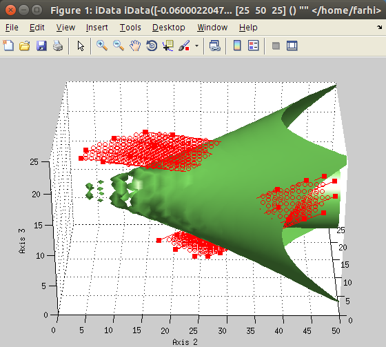
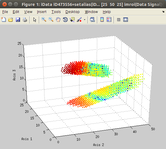
The
imroi selection tool allows to select polygonal
regions of interest (ROI, left).
Once extracted, the new data set can be plotted (right).
It is usual to have to select a region in data sets before e.g. fitting them, or alternatively, deselect some other parts ('odd' points). To do so, select the data sets to handle in the Data Sets list, then use the Data:Select Region of Interest (ROI) menu item. Then, simply click on the plot to define the polygonal region corresponding to the area you wish to keep in the data.
The corresponding mask (which has 1 where data is selected, and 0 elsewhere) will be added as a data set, which you may use further to multiply with some other data set. In addition, the same mask will be applied to all selected data sets (if more than one).
If you rather need to remove (deselect) some areas from your data set, use the Data:Deselect Region of Interest (ROI) menu item.
More help about this tool, and for instance to ability to define distinct areas in the same data set, or rotate the plot during selection, is available in the Plot page.
The selection functionality is also available from the Data:Transform:Unary operators menu item.
Mathematical operators on Data sets
It is possible to apply simple mathematical operators onto one or more Data Sets.
- Unary: these operators take single data sets, and return the same number of data sets after the transformation, which are appended to the Data Sets list. You can find typically: log, abs, trigonometric, opposite (uminus), ...
- Binary: these operators take operators two-by-two and return a single data set, which is appended to the Data Sets list. You can find typically:merge/combine, plus, minus, times, divide, comparisons, interpolation, FFT convolution, ...
- Others: these operators are usually specialized unary operators, and return the same number of data sets as the selected ones, which are appended to the Data Sets list. You can find typically: FFT, smoothing, intergral (trapz), cartesian to spherical/radial (cart2sph), wavelets (cwt), gradient and laplacian (del2), ...
For more complex treatment, you should retrieve the Data Sets in the Matlab/iFit workspace (prompt level), do some work, and send it back as new or updated Data sets. You can refer to the main iFit help page to learn what you can do, especially regarding the iData object handling, and Mathematical operators.
d=mifit('pull')set(d,'Model',gauss);d(1) = d(1)+d(2); % assuming we have selected 2 data sets.mifit('pull' d);
Working with Models (fitting)
You can use the available Models, which are listed in the Models menu, and sorted by dimensionality (1D,2D,...). You may import new models from files (including drag-n-drop), and from the Matlab/iFit prompt (which allows to create new Models). All Models are iFunc objects, and are saved in the miFit configuration (e.g. when exiting).
A detailed list of available models is given in the Models page.
| 1D models |
|
allometric Allometric/Freundlich (1D) [allometric]
bigauss Bi-Gaussian (1D) [bigauss]
bilorz Bi-Lorentzian (1D) [bilorz]
bose Bose (1D) [bose]
dho Damped-harmonic-oscillator (1D) [dho]
dirac Dirac (1D) [dirac]
doseresp Dose-response (sigmoid) (1D) [doseresp]
expon Exponential decay (1D) [expon]
expstretched Stretched Exponential decay (1D) [expstretched]
gauss Gaussian (1D) [gauss]
green Green function (1D) [green]
heaviside Heaviside (1D) [heaviside]
langevin Langevin function for magnetic polarization (1D) [langevin]
laplace Laplace distribution function (1D) [laplace]
lognormal Log-Normal distribution function (1D) [lognormal]
lorz Lorentzian (1D) [lorz]
maxwell Maxwell-Boltzmann *3 distribution function (1D) [maxwell]
pareto Pareto distribution distribution function (1D) [pareto]
| poisson Poisson distribution function (1D) [poisson]
powerlaw Power law (1D) [powerlaw]
pseudovoigt Pseudo-Voigt (1D) [pseudovoigt]
quadline Quadratic equation (1D) [quadline]
sigmoid Sigmoidal curve (1D) [sigmoid]
sine Sine function (1D) [sine]
sinedamp Damped-Sine function (1D) [sinedamp]
strline Straight-line (1D) [strline]
tophat Top-Hat rectangular function (1D) [tophat]
triangl Triangular function (1D) [triangl]
twoexp Bi-Exponential decay (1D) [twoexp]
voigt Voigt (1D) [voigt]
ff_core_shell Spherical/core shell P(q) (1D) [ff_core_shell]
ff_sphere Sphere P(q) (1D) [ff_sphere]
sf_hard_spheres Hard Sphere S(q) (1D) [sf_hard_spheres]
sf_square_well Square well S(q) (1D) [sf_square_well]
sf_sticky_hard_spheres Sticky Hard Sphere S(q) (1D) [sf_sticky_hard_spheres]
|
| 2D models |
lorz2d Lorenztian-2D function with tilt angle (2D) [lorz2d]
plane2d Planar function (2D) [plane2d]
pseudovoigt2d Pseudo-Voigt-2D function with tilt angle (2D) [pseudovoigt2d]
quad2d Quadratic-2D function with tilt angle (2D) [quad2d]
gauss2d Gaussian-2D function with tilt angle (2D) [gauss2d]
|
| 4D models |
sqw_acoustopt Sqw_acoustopt acoustic/optic dispersion(HKL) with DHO line shape [sqw_acoustopt]
sqw_cubic_monoatomic Sqw_cubic dispersion(HKL) for cubic monoatomic crystal [sqw_cubic_monoatomic]
sqw_linquad Sqw_linquad linear-quadratic dispersion(HKL) with DHO line shape [sqw_linquad]
sqw_sine3d Sqw_sine3d sine dispersion(HKL) with DHO line shape [sqw_sine3d]
sqw_phonons Sqw_phonon DHO [sqw_phonons]
sqw_spinw Sqw_spinw spin-wave dispersion(HKL) [sqw_spinw]
sqw_vaks Sqw_Vaks phonon dispersion(HKL) for perovskites ABX3 [sqw_vaks]
|
Other models
|
constant Constant (0D) [constant]
gaussnd Gaussian (nD) [gaussnd]
ngauss Gaussians_n (n*1D) [ngauss]
nlorz Lorentzians_n (n*1D) [nlorz]
rietveld Rietveld refinement [rietveld]
|
Assigning and Evaluating Models to Data sets
You should first select the target Data Set(s) in the list, which will be assigned a given model. Then, select a model from the Models menu (1D,2D, ....).
To view the Model Parameters, select the View Model Parameters item in the Models menu. This window has a contextual menu which provides additional features (e.g. on right-click or Ctrl-click).

The miFit Model Parameters window. You can fix and set parameter bounds.
When selecting many Data Sets, and changing a parameter in the Model Parameter Window, all data sets are affected (e.g if you change the Amplitude parameter, all parameters with same name in data sets will be changed. This allows to quickly set common parameters to many data sets and models.
Also, when a plot for current data sets is visible, and the evaluation of the model is faster than 0.5 s, the model will be evaluated and updated on plots every time a parameter is changed.
You can force to evaluate the Model onto selected Data Set axes from the Evaluate Model in the Data menu. When no model parameters have been set yet, the model will guess some starting parameters from the data set.
To force an update of the Model Parameter Window (with e.g. guessed values), de-select (Ctrl-click or click an other data set) and re-select (click) the Data Set from the list.
Plotting one or more Data Set with assigned models will also display their model evaluation (see above).
Selecting a fit routine (optimization algorithm)
The default choices for the optimizer and the fit criteria will 'work' in most cases. However, you may specifically select the optimizer, its configuration, the fit criteria and the verbosity level (for interactive actions).
The optimizer to be used for fitting can be chosen from the Optimizers menu. The 'Automatic best optimizer'
(fmin) makes a reasonable choice among all available optimizers,
depending on the model dimensionality. This is the default choice.
However, you may choose any of the available optimizers (see Optimizers for a more detailed description). More specifically, we recommend the 'Particle Swarm Optimization [fminpso]' which may be longer to converge, but is one of the most robust, meaning it will do a global search and can hardly be trapped in local minima, as do most gradient based optimizers.
- Configuration of the algorithm: The configuration of the optimizer allows to change the internal optimizer parameters, such as the number of iterations, the desired accuracy (convergence criteria), ... The default configuration should work in most cases.
- Selecting the optimization criteria (least-squares, ...): use the Select Criteria entry in the Optimizers menu. Usual choice is least-square, but other choices are possible. Refer to the Fit help page for more.
- Selecting the optimizer: Select one entry in the Optimizers menu. Use for instance the 'Automatic best [fmin]' or e.g. 'Particle Swarm Optimization [fminpso]'. Refer to the Optimizers page.
- The verbose mode: in the Preferences from the File menu, you can turn the Verbosity item from 'no' to 'yes' to follow the fit procedure. During the fit, the criteria evolution, as well as the data and model evaluation plot will displayed. The View Parameters window will also be regularly updated. You can also click the Stop red button during the fit to cleanly interrupt the procedure.
Fitting Models to Data sets
Once a data set has been assigned a model, it is possible to fit the model parameters onto the data. The procedure makes use of the following concepts:
- the model is also called the 'objective' function ;
- the model parameters are changed during the fit procedure so that the model evaluated with these parameters converges as best as possible to the data set. The number of parameters is the problem dimensionality. The number of degrees of freedom is the number of data set points minus the number of parameters ;
- the metric used to compare the data set and the model evaluation during the fit is called the 'criteria' . It is often defined as the least-square, but other choices are possible ;
- the procedure used to perform the fit is called the 'optimizer' (see Optimization). Known optimizers are the Levenberg-Marquardt, the swarm (particules), the simplex, etc...
The fit process is launched when selecting the Fit to Model item of the Data menu, or clicking the fit icon in the toolbar. The model parameters will be changed according to the selected optimizer strategy, in order to minimise the criteria, which is a function to measure the distance between the data set and the model.
WARNING: it is highly recommended to bound the model parameters, to help the optimizer find reasonable values, and speed-up the whole process. Leaving completely unbound parameters may result in non-sensible final values. Also, it is better to reduce as much as possible the number of free parameters.
The Fit_Verbose mode ('yes') in the Preferences allows to follow the fit procedure and to be able to interrupt it cleanly during the fit (Stop button). However, the procedure is significantly slower, as displaying the updates at every iteration takes more time. The Fit_Verbose=yes option is highly recommended. It consists in:
- Update the model parameter values in the model Parameter window.
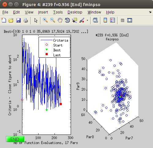
- Update the plot showing the data, the model, and the best match.
- Show the criteria evolution, aside the parameter space.
- Provide a clean STOP button to end the fit procedure.
- Display the distributions for all model parameter at the end (can also be generated from the Parameter window contextual menu).
When not in verbose mode, the Fit procedure still displays a simple STOP button that you can click to abort.
Preferences
The miFit Preferences window. The Preferences are updated and saved when closing the window. To Reset Preferences, use the File:Reset menu item.
The miFit Preferences allow to customize the behaviour of miFit. You can more specifically change the font size (use e.g. 16 on high DPI monitors), or the verbosity level. Additional menu are also stored there, and are usually generated from a predefined configuration (File:Configurations menu item).
In case you are behind a proxy, you can also set here its address and port. Do not use a full URL for the proxy, e.g. do not specify 'http://proxy.ill.fr' but rather 'proxy.ill.fr'. The port should be a valid number [0-9999], e.g. 8888. To remove a proxy setting, set it to empty.
Resetting miFit (default Preferences)
To Reset the miFit application, use the Reset item in the File menu. The 'Reset' button will clear the data set list, History and Log file. The Factory reset will also clear the Models list (menu), and Preferences. This last choice requires miFit to be restarted in order to be effective. Specific menus from the File:Configurations are also removed.
Saving your work
Saving all data sets, Models and Preferences
Use the Save item in the File menu to save the Data Sets, Models, and Optimizers, e.g. in the mifit.mat file in the Matlab Preferences directory. This file is automatically re-opened when starting miFit, so that the last configuration is fully restored from one session to an other.
You may as well save this information into a specific file, using the Save as item in the File menu. You can then later re-open this file from the Open item in the File menu.
Preferences are saved automatically. They are restored when starting a new miFit session. The location of this file is indicated in the dialog, and in the console. You may make copies of this file for later restore. The File:Configurations menu item corresponds with predefined settings (.ini files, including new menus to appear in the interface) stored in the 'configurations' directory in the miFit installation.
In addition, you can also look at the content of the mifit Log file (menu item File:Show Log...) which saves most of the application operations. This file can be either removed manually, or using the File:Reset menu item.
Exporting selected Data sets
Into files
Use the Data:Export menu item to export the selected data sets into a number of formats, as detailed in the Save page.
The recommended formats for export are: Matlab MAT, HDF/NeXus, Hypertext HTML, Flat text DAT.
We also recommend JSON and YAML formats, but the generated files may be large. You may eventually compress them using e.g. ZIP.
The HTML export format includes links to other common data formats, and is thus one of our recommended formats.
The Matlab MAT format generated using this method is serialized. It is extremely fast to read/write, but is not fully portable. You need to e.g. import it with miFit/iFit to recover the data set. To get a 'regular' Matlab MAT, use the File:Save and File:Save as menu items.
Data Set Export formats (recommended in bold)
|
|
CDF (*.cdf)
Comma Separated Values (suitable for Excel, *.csv)
Flat text file with comments (*.dat)
EDF ESRF format for 1D and 2D data sets (*.edf)
Encapsulated PostScript (color, *.eps)
Matlab figure (*.fig)
IAU FITS binary image (*.fits, only for 2D objects)
Hierarchical Data Format 5 (*.hdf5, *.h5, *.hdf)
Hierarchical Data Format 4 image (*.hdf4)
Analyze volume (*.hdr+img)
Hypertext Markup Language document (*.html)
JPEG image (*.jpg)
JSON JavaScript Object Notation (*.json)
Matlab script/function (*.m)
Matlab binary file (*.mat, serialized)
MRC map file (*.mrc)
NetCDF (*.nc, *.cdf)
NiFti volume (*.nii)
| Object File Format geometry (*.off)
PLY geometry (*.ply)
Portable Document Format (*.pdf)
PostScript (color, *.ps)
Portable Network Graphics image (*.png)
Portable Anymap format (*.pnm)
Stereolithography geometry (*.stl)
Scalable Vector Graphics (*.svg)
TIFF image (*.tif)
VTK volume (*.vtk)
Virtual Reality file (*.wrl, *.vrml)
X3D (geometry) file, ascii (*.x3d)
embedded HTML/X3D file (*.html using Flash plugin for rendering)
Excel format (requires Excel to be installed, *.xls)
XML file (*.xml)
YAML interchange format (*.yaml) |
You can also save the Data Sets as a miFit Matlab (*.mat) file with the File:Save and File:Save as menu items, or the 'save' icon in the toolbar. Such MAT files are 'regular' Matlab workspace files.
Most generated files can be re-imported into miFit.
To the Matlab/iFit prompt
You can send the current selected Data Sets from the miFit interface to the command prompt using:
which will either be a single iData object, possibly with a 'Model' alias, or an array of such objects if the selection contains more than one item.
To get all data sets, use:
The resulting variable, here 'd', can be processed with any of the iData methods (including Math stuff).
You can send back the modified objects, either as new data sets with:
or replacing/updating existing data sets, with:
in which case new data sets are appended to the miFit list.
Copy/Paste
Using the File:Edit or e.g. Ctrl-C key (command-C on MacOSX), you can transfer one or more Data Sets into the clipboard, and to other applications. The format of the clipboard is a formatted text containing identification items, and the data set values. The whole content of the Data Set (e.g. model and other attached data) is not full copied.
As table
Selected data sets can be viewed as tables, which opens for each data set an Excel-like spreadsheet. You can modify the data set values, and access a contextual menu with Ctrl-Click to e.g.:
- export to Excel CSV
- copy/paste to/from the clipboard
- resize the data set (crop or extend)
- plot a selection
Large data sets may be slow to render, and should be used with data containing e.g. up to few thousand elements.
As web pages (for printing)
The File:Print and the 'printer' icon in the toolbar allow to generate a document ready for printing, displayed in a web browser. As opposed to the Data:Export with HTML format (see above), which includes a number of data formats, the Print feature displays a simplified version of the Data Set(s), which is faster to generate.
Exporting Models (and importing them as well
Models generated by the user (displayed in blue or green in the Models menu) can be exported. Use the Models:Export menu item, and select one of the available formats.
The recommended formats for export are: Matlab M or MAT, JSON and YAML.
| Models Export formats (recommended in bold) |
|
Flat text file with comments (*.dat)
Encapsulated PostScript (color, *.eps)
Matlab figure (*.fig)
Hierarchical Data Format 4 image (*.hdf4)
Hypertext Markup Language document (*.html)
JPEG image (*.jpg)
JSON JavaScript Object Notation (*.json)
| Matlab script/function (*.m)
Matlab binary file (*.mat)
Portable Document Format (*.pdf)
Portable Network Graphics image (*.png)
PostScript (color, *.ps)
TIFF image (*.tif)
XML file (*.xml)
YAML interchange format (*.yaml) |
You can edit, and re-import these files within miFit with the Models:Import menu item.
Examples / Tutorials
Fitting a simple peak
In this example, we demonstrate how to fit a simple data set with a Gaussian model.
 Import a TAS data file. This is e.g. a Q or Energy scan. You may for instance get the MnFeSi_0099.scn file as example (drag-and-drop it into miFit, navigate to it with the File:Open selector, or copy-paste its path). Double click it to view the data set.
- Select the Models:1D:Gaussian model. The Parameter window pops-up, no parameter value is set.
- Click on the Data:Evaluate Model or the 'fx' icon in the toolbar. Guessed parameters are then used. To update these in the Parameter window, use Ctrl-click twice on the Data set (de-select and re-select).
- Bound the Amplitude between 0 and 0.002, the Centre in [0.1 and 0.2], the HalfWidth between 0 and .2, the Background in [0 1e-3]. Every time you change some model Parameter setting, the plot is updated.
- Choose the Levenberg-Marquardt [fminlm] optimizer.
- Set the Fit_Verbose to 'no' in the File:Preferences.
- Finally, click on the Fit icon in the toolbar, or select Data:Fit.
- Double-click the Data Set to plot it and display the fit result.
- Use Edit:Undo twice, and re-select the Data Set. The initial model parameters are restored.
- Set the Fit_Verbose to 'yes' in the File:Preferences.
- Click again on the Fit icon. You see that the fit is much slower, as all windows are updated at every iteration. The criteria, plot, and parameter space are all updated during the fit. A STOP button allows to abort the fit.
- At the end of the fit, the parameter distributions are displayed.
Fitting a 'phonon' dispersion (neutron_TAS)
We here indicate the usual steps to be used to treat a TAS scan around a dispersion.
- Import a TAS data file. This is e.g. a Q or Energy scan. You may for instance get the MnFeSi_0099.scn file as example (drag-and-drop it into miFit, navigate to it with the File:Open selector, or copy-paste its path). Double click it to view the data set. This is a vector data set (signal as a function of QL), so 1D.
- Install the Neutron Scattering menu with TAS plug-ins but selecting the File:Configurations:neutron_TAS.ini
- Select the data file, and convert it to a 4D (QH QK QL EN) scan, using the TAS: Convert/Convolute 4D item in the Neutron Scattering menu. As there is no Model assigned, only the data set in converted to 4D. A new item appears in the Data sets list.
- Assign a 4D model, e.g. sqw_linquad which models a local S(q,w) description around e.g. the scan center.
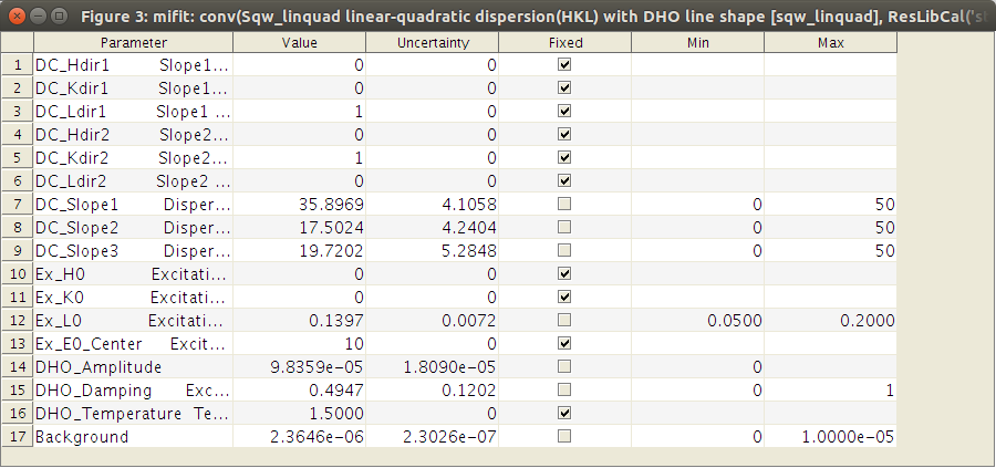 Open the View Parameters window by selecting the View Model Parameters item in the Models menu.
- Set initial model parameters (e.g. excitation energy). Make sure to fix e.g. HKL space directions and some other parameters to help the fit to converge. Bound parameters (e.g. excitation energy and Q location...). Adjust Amplitude and Damping. For this model, make sure that the linear direction DC_dir1 matches the actual TAS scan direction. With the example data file, the scan is along QL, which is a rather 'linear' branch. Then the DC_dir1 should be along QL, i.e. [0 0 1]. The quadratic direction should be perpendicular (can be left unchanged).
- Optionally, turn Fit_Verbosity to 'yes' in the File:Preferences (recommended), which allows to follow the fit procedure, and stop it any time.
- Click on the Fit icon or item in the Data menu. This first fit is an ideal one, without the 4D convolution with the neutron TAS resolution. It will probably not fit the peak width, as most of the effect originates from the spectrometer resolution.
- Now, open the ResLibCal interface from the Neutron Scattering menu.
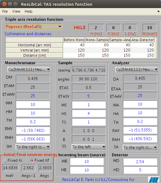
- Optionally import a data file, previous or predefined instrument configuration in ResLibCal to read the spectrometer configuration. This data file should contain Rescal parameters in free text. You can also check/modify instrument and sample parameters in its main window. If you do not import a TAS configuration, you can still configure the parameters in the ResLibCal interface, or the last saved configuration will be used. In this example, we suggest that you open the MnFeSi_0099.scn filewith ResLibCal to initiate the instrument configuration. Check carefully the instrument parameters. Once done, we also suggest that you save your tuned instrument configuration into a .ini format file (ResLibCal File:Save as menu item) so that you can re-use it later.
- Select the method to compute the resolution from Cooper-Nathans, Popovici or McStas full Monte-Carlo. The resolution uses a Monte-Carlo cloud for the 4D convolution operation which creates a set of points around each TAS measurement location. The resolution
is re-computed at each location. The number of points used in this
cloud is defined in the ResLibCal View:Set Monte-Carlo iterations item. We recommend the Popovici method as a start (top left corner of the ResLibCal GUI).
- In miFit select the 4D data set (QH QK QL EN), and convolve the model with the 4D TAS resolution function, using (again) the TAS: Convert/Convolute 4D item in the Neutron Scattering menu. This time, the assigned model is affected.
- You can optionally close ResLibCal (which saves the current configuration to be used). This makes the fit procedure slightly faster, using the last saved configuration. We recommend to keep ResLibCal opened, as it is then easy to change the TAS configuration from one fit to an other.
 Optionally: select a specific Optimizer from the same menu in miFit. We recommend the Particle Swarm Optimization [fminpso] which is very robust.

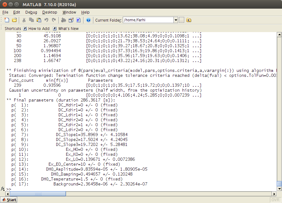
 Click on the Fit icon or item in the Data menu.The fit steps are printed into the Matlab/iFit prompt.
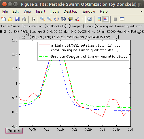
- The evolution of the Fit criteria (here least-squares) is displayed during the fit as a function of the number of model evaluations, as well as the space of the three first varying parameter. The Model Parameter window is updated with the on-going values, as well as a plot showing the comparison between the data set, the model, and the best parameter set found so-far.
 At the end of the fit, the final parameter values are displayed in the Parameter window, in the command/prompt, with the attached uncertainty. The parameter distribution is also shown, in the style of a Markov chain result. [Red distributions indicate parameters which have been found highly correlated to others (non-independent)]
- You can close most plots, and update the initial Data Set plot (see step 1). The final model parameters and evaluation are stored into the data set. The Parameter distribution (Markov-style) can be obtained from the Model Parameter window, contextual menu.


 The miFit File menu has an Evaluate code/script menu item. Your can enter any Matlab command there, and evaluate a selection, or all ('Play' button or the TextEdit:File:Evaluate selection item) . To send some data directly to miFit, use e.g.:
 You can plot Data Sets by selecting one or more, and then click on the Plot icon in the toolbar, or the Plot item in the Data menu. To plot a single Data Set, double-click it in the Data Set list. Data Sets with assigned Models (see below) will also show the model evaluation.


 Import a TAS data file. This is e.g. a Q or Energy scan. You may for instance get the MnFeSi_0099.scn file as example (drag-and-drop it into miFit, navigate to it with the File:Open selector, or copy-paste its path). Double click it to view the data set.
 Open the View Parameters window by selecting the View Model Parameters item in the Models menu.
 Optionally: select a specific Optimizer from the same menu in miFit. We recommend the Particle Swarm Optimization [fminpso] which is very robust.
 Click on the Fit icon or item in the Data menu.The fit steps are printed into the Matlab/iFit prompt.
 At the end of the fit, the final parameter values are displayed in the Parameter window, in the command/prompt, with the attached uncertainty. The parameter distribution is also shown, in the style of a Markov chain result. [Red distributions indicate parameters which have been found highly correlated to others (non-independent)]